UNIT-5

Partial differential equation: Higher order

5.1 Classification of Second order partial differential equations

The second order PDE in two independent variables of the form

Here a,b,c,d,e,f and g are the functions of the independent variables x and y.

The principal part of the operator L, can be given as-

The equation is classified as-

Hyperbolic if-

Parabolic if-

Elliptic if-

Here is the discriminant of the operator L.

Example: Classify the following PDEs into hyperbolic, parabolic or elliptic.

Sol. In the first PDE, a = 1, b = 0 and c =

So that-

Thus we can say that the given PDE is hyperbolic.

Now in second PDE,

A = 1, b = 0 and c =

So that-

Therefore the second PDE is elliptic.

5.2  Separation of variables method to simple problems in Cartesian coordinates including two dimensional Laplace, one dimensional Heat and one dimensional Wave equations

Method of separation of variables

In this method, we assume that the dependent variable is the product of two functions, each of which involves only one of the independent variables. So to ordinary differential equations are formed.

Example 1. Using the method of separation of variables, solve

Solution. 

Let, u = X(x). T (t).                     (2)

Where X is a function of x only and T is a function of t only.

Putting the value of u in (1), we get

(a) 

On integration log X = cx + log a = log

(b)

On integration

Putting the value of X and T in (2) we have

But,

i.e.

Putting the value of a b and c in (3) we have

Which is the required solution.

Example 2. Use the method of separation of variables to solve equation

Given that v = 0 when t→ as well as v =0 at x = 0 and x = 1.

Solution.

Let us assume that v = XT where X is a function of x only and T that of t only

Substituting these values in (1), we get

Let each side of (2) equal to a constant

Solving (3) and (4) we have

Putting x = 0, v = 0 in (5) we get

On putting the value of in (5) we get

Again putting x = l, v= 0 in (6) we get

Since cannot be zero.

Inputting the value of p in (6) it becomes

Hence,

This equation satisfies the given condition for all integral values of n. Hence taking n = 1, 2, 3,… the most general solution is

Example. Using the method of separation of variables, solve Where

Solution. Assume the given solution

Substituting in the given equation, we have

Solving (i)

From (ii)

Thus

Now,

Substituting these values in (iii) we get

Which is the required solution

The Laplacian in plane

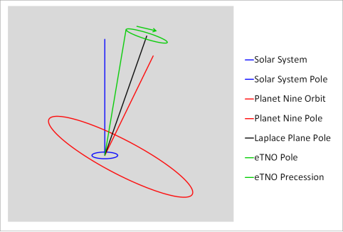
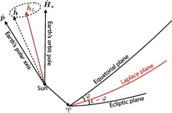
The axis of Laplace plane is coplanar with, and between,

(a) The polar axis of the parent planet's spin, and

(b) The orbital axis of the parent planet's orbit around the Sun.

The Laplace plane arises because the equatorial oblateness of the parent planet tends to cause the orbit of the satellite to precess around the polar axis of the parent planet's equatorial plane, while the solar perturbations tend to cause the orbit of the satellite to precess around the polar axis of the parent planet's orbital plane around the Sun. The two effects acting together result in an intermediate position for the reference axis for the satellite orbit's precession.

The mean plane occupied by the orbit of a satellite during a precession cycle; the plane normal to the orbital precession pole of the satellite.

In effect, this is the plane normal to the orbital precession pole of the satellite. It is a kind of "average orbital plane" of the satellite, around which the instantaneous orbital plane of the satellite precesses, and to which it has a constant additional inclination.

In most cases, the Laplace plane is very close to the equatorial plane of its primary planet (if the satellite is very close to its planet) or to the plane of the primary planet's orbit around the Sun (if the satellite is far away from its planet). This is because the strength of the planet's perturbation on the satellite's orbit is much stronger for orbits close to the planet, but drops below the strength of the Sun's perturbation for orbits farther away.

Examples of satellites whose Laplace plane is close to their planet's equatorial plane include the satellites of Mars and the inner satellites of the giant planets. Examples of satellites whose Laplace plane is close to their planet's orbital plane include Earth's Moon and the outer satellites of the giant planets. Some satellites, such as Saturn's Iapetus, are situated in the transitional zone and have Laplace planes that are midway between their planet's equatorial plane and the plane of its solar orbit.

So the varying positions of the Laplace plane at varying distances from the primary planet can be pictured as putting together a warped or non-planar surface, which may be pictured as a series of concentric rings whose orientation in space is variable: the innermost rings are near the equatorial plane of rotation and oblateness of the planet, and the outermost rings near its solar orbital plane. Also, in some cases, larger satellites of a planet (such as Neptune's Triton) can affect the Laplace planes of smaller satellites orbiting the same planet.

Duhamel's principle for one dimensional wave equation

One dimensional heat flow

Let heat flow along a bar of uniform cross section in the direction perpendicular to the cross section. Take one end of the bar as origin and the direction of the heat flow is along x axis.

Let the temperature of the bar at any time t at a point x distance from the origin be u(x,t). Then the equation of one dimensional heat flow is

Example 1. A rod of length 1 with insulated sides is initially at a uniform temperature u. Its ends are suddenly cooled to 0° Celsius and are kept at that temperature. Prove that the temperature function u (x, t) is given by

Where is determined from the equation.

Solution. Let the equation for the conduction of heat be

Let us assume that u = XT, where X is a function of x alone and T that of t alone.

Substituting these values in (1) we get

i.e.

Let each side be equal to a constant

And

Solving (3) and (4) we have

Putting x = 0, u = 0 in (5), we get

(5) becomes

Again putting x = l, u =0 in (6), we get

Hence (6) becomes

This equation satisfies the given conditions for all integral values n. Hence taking n = 1, 2, 3,…, the most general solution is

By initial conditions

Example 2. Find the solution of

For which u ( 0, t) = u (l.t) =0 =sin bi method of variable separable.

Solution.

In example 10 the given equation was

On comparing (1) and (2) we get

Thus solution of (1) is

On putting x =0

u =0 in (3) we get

(3) reduced to

On putting x = l and u =0 in (4) we get

Now (4) is reduced to

On putting t = 0, u =

This equation will be satisfied if

On putting the values of and n in (5) we have

Example 3. The ends A and B of a rod 20 cm long having the temperature at 30 degree Celsius and at 80 degree Celsius until steady state prevails. The temperature of the ends are changed to 40 degree Celsius and 60 degree Celsius respectively. Find the temperature distribution in the rod at time t.

Solution. The initial temperature distribution in the rod is

And the final distribution (i.e. steady state) is

To get u in the intermediate period, reckoning time from the instant when the end temperature were changed we assumed

Where is the steady state temperature distribution in the rod (i.e. temperature after a sufficiently long time) and is the transient temperature distribution which tends to zero as t increases.

Thus,

Now satisfies the one dimensional heat flow equation

Hence u is of the form

Since

Hence

Using the initial condition i.e.

Putting this value of n (1), we get

D Alembert’s solution of the one dimensional wave equation

The method of d'Alembert provides a solution to the one-dimensional wave equation

That models vibrations of a string.

The general solution can be obtained by introducing new variables  and , and applying the chain rule to obtain

Using (4) and (5) to compute the left and right sides of (3) then gives

Respectively, so plugging in and expanding then gives

This partial differential equation has general solution

Where f and g are arbitrary functions, with f representing a right-traveling wave and g a left-traveling wave.

The initial value problem for a string located at position  as a function of distance along the string x and vertical speed  can be found as follows. From the initial condition and (12),

Taking the derivative with respect to  then gives

And integrating gives

Solving (13) and (16) simultaneously for f and g immediately gives

So plugging these into (13) then gives the solution to the wave equation with specified initial conditions as

Example. Find the deflection of a vibrating string of unit length having fixed ends with initial velocity zero and initial deflection f (x)=k (sinx –sin2x)

Solution. By d’Alembert’s method, the solution is

i.e., the given boundary corrections are satisfied.