Unit II
Measures of Central Tendency
A measure of central tendency is a statistical summary that represents the center point of the dataset. It indicates where most values in a distribution fall. It is also called as measure of central location.
The three most common measure of central tendency are Mean, Median, and Mode.
According to Prof Bowley “Measures of central tendency (averages) are statistical constants which enable us to comprehend in a single effort the significance of the whole.”
Requisites of a good measure of central tendency
1. It should be rigidly defined
2. It should be simple to understand and easy to calculate
3. It should be based upon all values of given data.
4. It should be capable of further mathematical treatment.
5. It should have sampling stability.
6. It should be not be unduly affected by extreme values.


2.2.1 Median:
- The points or value that divides the data into two equal parts
- Firstly, the data are arranged in ascending or descending order .
- The median is the middle number depending on the data size.
- When the data size is odd, the median is the middle value
- When the data size is even, median is the average of the middle two values
 It is also known as middle score or 50th percentile
For ungrouped data median is calculated by  value
value
Example 1– find the median score of 7 students in science class
Score = 19, 17, 16, 15, 12, 11, 10
Median = (7+1)/2 = 4th value
Median = 15
Find the median score of 8 students in science class
Score = 19, 17, 16, 15, 12, 11, 10, 9
Median = (8+1)/2 = 4.5th value
Median = (15+12)/2 = 13.5
Example 2 – find the median of the table given below
Marks obtained | No. Of students |
20 | 6 |
25 | 20 |
28 | 24 |
29 | 28 |
33 | 15 |
38 | 4 |
42 | 2 |
43 | 1 |
Solution
Marks obtained | No. Of students | Cf |
20 | 6 | 6 |
25 | 20 | 26 (20+6) |
28 | 24 | 50 (26+24) |
29 | 28 | 78 |
33 | 15 | 93 |
38 | 4 | 97 |
42 | 2 | 99 |
43 | 1 | 100 |
Median = (n+1)/2 = 100+1/2 = 50.5
Median = (28+29)/2 = 28.5
Median of grouped data
Formula

 MC = median class is a category containing the n/2
Lb = lower boundary of the median class
Cfp = cumulative frequency before the median class if the scores are arranged from lowest to highest value
Fm = frequency of the median class
c.i = size of the class interval
Ex- calculate the median
Example 3-
Calculate the median
Marks | No. Of students |
0-4 | 2 |
5-9 | 8 |
10-14 | 14 |
15-19 | 17 |
20-24 | 9 |
Solution
Marks | No. Of students | CF |
0-4 | 2 | 2 |
5-9 | 8 | 10 |
10-14 | 14 | 24 |
15-19 | 17 | 41 |
20-24 | 9 | 50 |
| 50 |
|
n = 50
 n = 50/2= 25
2
The category containing n/2 is 15 -19
Lb = 15
Cfp = 24
f = 17
Ci = 4


 Median = 15 + 25-24 *4 = 15.23
17
Example 4 - Given the below frequency table calculate median
X | 60 – 70 | 70 – 80 | 80- 90 | 90-100 |
F | 4 | 5 | 6 | 7 |
Solution
X | F | CF |
60 - 70 | 4 | 4 |
70 - 80 | 5 | 9 |
80 - 90 | 6 | 15 |
90 - 100 | 7 | 22 |
n = 22
 n = 22/2= 11
2
The category containing n+1/2 is 80 - 90
Lb = 80
Cfp = 9
f = 6
Ci = 10


 Median = 80 + 11-9 *10 = 83.33
6
Example 5– calculate the median of grouped data
Class interval | 1-3 | 3-5 | 5-7 | 7-9 | 9-11 | 11-13 |
Frequency | 4 | 12 | 13 | 19 | 7 | 5 |
Solution
CI | F | CF |
1-3 | 4 | 4 |
3-5 | 12 | 16 |
5-7 | 13 | 29 |
7-9 | 19 | 48 |
9-11 | 7 | 55 |
11-13 | 5 | 60 |
n = 60
 n = 60/2= 30
2
The category containing n+1/2 is 7-9
Lb = 7
Cfp = 29
f = 19
Ci = 2


 Median = 7 + 30-29 *2 = 7.105
19
Merits of median
- It is rigidly defined
- It is easy to understand and easy to calculate
- It is not affected by extreme values
- It is not much affected by sampling fluctuation
- It can be located graphically
Demerits of median
- It is not based upon all values of the given data
- It is difficult to calculate increasing order data size
- It is not capable of further mathematical treatment.
2.2.2 Mode:
- The mode is denoted Mo, is the value which occurs most frequently in a set of values.
- Croxton and Cowden defined it as “the mode of a distribution is the value at the point armed with the item tends to most heavily concentrated. It may be regarded as the most typical of a series of value”
Mode for ungrouped data
Example 1- Find the mode of scores of section A
Scores = 25, 24, 24, 20, 17, 18, 10, 18, 9, 7
Solution – Mode is 24, 18 as both have occurred twice.
Mode for grouped data
 Mode = L1 + (L2 – L1) d1
d1 +d2
L1= lower limit of the modal class,
L2= upper limit of the modal class‟
d1 =fm-f0 and d2=fm-f1
Where fm= frequency of the modal class,
f0 = frequency of the class preceding to the modal class,
f1= frequency of the class succeeding to the modal class.
Example 2 – find the mode
Seconds | Frequency |
51 - 55 | 2 |
56 - 60 | 7 |
61 - 65 | 8 |
66 - 70 | 4 |
The group with the highest frequency is the modal group: - 61-65
D1 = 8-7 = 1
D2 = 8-4 = 4
 Mode = L1 + (L2 – L1) d1
d1 +d2
 mode = 61 + (65-61) 1 = 61+4 (1/5) = 61.8
1+4
Mode = 61.8
Example 3 - In a class of 30 students marks obtained by students in science out of 50 is tabulated below. Calculate the mode of the given data.
Marks obtained | No. Of students |
10 -20 | 5 |
20 – 30 | 12 |
30 – 40 | 8 |
40 - 50 | 5 |
Solution
The group with the highest frequency is the modal group: - 20 -30
D1 = 12 - 5 = 7
D2 = 12 - 8 = 4
 Mode = L1 + (L2 – L1) d1
d1 +d2
 mode = 20 + (30-20) 7 = 20+10 (7/11) = 26.36
7+4
Mode = 61.8
Example 4- Based on the group data below, find the mode
Time to travel to work | Frequency |
1 – 10 | 8 |
11 -20 | 14 |
21 – 30 | 12 |
31 – 40 | 9 |
41 - 50 | 7 |
Solution
The group with the highest frequency is the modal group: - 11 - 20
D1 = 14 - 8 = 6
D2 = 14 - 12 = 2
 Mode = L1 + (L2 – L1) d1
d1 +d2
 mode = 11 + (20-11) 6 = 11+9 (6/8) = 17.75
6+2
Example 5 –
Compute the mode from the following frequency distribution
CI | F |
70-71 | 2 |
68-69 | 2 |
66-67 | 3 |
64-65 | 4 |
62-63 | 6 |
60-61 | 7 |
58-59 | 5 |
Solution
The group with the highest frequency is the modal group: - 60 - 61
D1 = 7 - 6 = 1
D2 = 7 - 5 = 2
 Mode = L1 + (L2 – L1) d1
d1 +d2
 mode = 60 + (61-60) 1 = 60+1 (1/3) 60.85
1+2
Merits of mode
- It is easy to understand & easy to calculate
- It is not affected by extreme values or sampling fluctuations.
- Even if extreme values are not known mode can be calculated.
- It can be located just by inspection in many cases.
- It is always present within the data.
Demerits of mode
- It is not rigidly defined.
- It is not based upon all values of the given data.
- It is not capable of further mathematical treatment.
2.2.3 Arithmetic Mean:
- The mean is the arithmetic average, also called as arithmetic mean.
- Mean is very simple to calculate and is most commonly used measure of the center of data.
- Means is calculated by adding up all the values and divided by the number of observations.
Computation of sample mean -
If X1, X2, ………………Xn are data values then arithmetic mean is given by

Computation of the mean for ungrouped data

Example 1 – The marks obtained in 10 class test are 25, 10, 15, 30, 35


 The mean = X = 25+10+15+30+35 = 115 =23
5 5
Analysis – the average performance of 5 students is 23. The implication that students who got below 23 did not perform well. The students who got above 23 performed well in exam.
Example 2 – find the mean
Xi | 9 | 10 | 11 | 12 | 13 | 14 | 15 |
Freq (Fi) | 2 | 5 | 12 | 17 | 14 | 6 | 3 |
Xi | Freq (Fi) | XiFi |
9 | 2 | 18 |
10 | 5 | 50 |
11 | 12 | 132 |
12 | 17 | 204 |
13 | 14 | 182 |
14 | 6 | 84 |
15 | 3 | 45 |
| Fi = 59 | XiFi= 715 |
|
|
|
Then, N = ∑ fi = 59, and ∑fi Xi=715
 X = 715/59 = 12.11
Mean for grouped data
Grouped data are the data that are arranged in a frequency distribution
Frequency distribution is the arrangement of scores according to category of classes including the frequency.
Frequency is the number of observations falling in a category
The formula in solving the mean for grouped data is called midpoint method. The formula is

 Where,X = Mean
Xm = midpoint of each class or category
f = frequency in each class or category
∑f Xm = summation of the product of fXm
Example 3– the following data represent the income distribution of 100 families. Calculate mean income of 100 families?
Income | 30-40 | 40-50 | 50-60 | 60-70 | 70-80 | 80-90 | 90-100 |
No. Of families | 8 | 12 | 25 | 22 | 16 | 11 | 6 |
Solution
Income | No. Of families | Xm (Mid point) | FXm |
30-40 | 8 | 35 | 280 |
40-50 | 12 | 34 | 408 |
50-60 | 25 | 55 | 1375 |
60-70 | 22 | 65 | 1430 |
70-80 | 16 | 75 | 1200 |
80-90 | 11 | 85 | 935 |
90-100 | 6 | 95 | 570 |
| n = 100 |
| ∑f Xm = 6198 |

X = ∑f Xm/n = 6330/100 = 63.30
Mean = 63.30
Example 4 –calculate the mean number of hours per week spent by each student in texting message.
Time per week | 0 - 5 | 5 - 10 | 10 - 15 | 15 - 20 | 20 - 25 | 25 – 30 |
No. Of students | 8 | 11 | 15 | 12 | 9 | 5 |
Solution
Time per week (X) | No. Of students (F) | Mid point X | XF |
0 - 5 | 8 | 2.5 | 20 |
5 – 10 | 11 | 7.5 | 82.5 |
10 - 15 | 15 | 12.5 | 187.5 |
15 - 20 | 12 | 17.5 | 210 |
20 - 25 | 9 | 22.5 | 202.5 |
25 – 30 | 5 | 27.5 | 137.5 |
| 60 |
| 840 |
Mean = 840/60 = 14
Example 5 –
The following table of grouped data represents the weights (in pounds) of all 100 babies born at a local hospital last year.
Weight (pounds) | Number of Babies |
[3−5) | 8 |
[5−7) | 25 |
[7−9) | 45 |
[9−11) | 18 |
[11−13) | 4 |
Solution
Weight (pounds) | Number of Babies | Mid point X | XF |
[3−5) | 8 | 4 | 32 |
[5−7) | 25 | 6 | 150 |
[7−9) | 45 | 8 | 360 |
[9−11) | 18 | 10 | 180 |
[11−13) | 4 | 12 | 48 |
| 100 |
| 770 |
Mean = 770/100 = 7.7
Merits of mean
- It is rigidly defined
- It is easy to understand and easy to calculate
- It is based upon all values of the given data
- It is capable of future mathematical treatment
- It is not much affected by sampling fluctuation
Demerits of mean
- It cannot be calculated if any observation are missing
- It cannot be calculated for open end classes
- It is effected by extreme values
- It cannot be located graphically
- It may be number which is not present in the data
2.2.4 Geometric Mean:
Geometric mean is a type of mean or average, which indicates the central tendency of a set of numbers by using the product of their values.
Definition
The Geometric Mean (G.M) of a series containing n observations is the nth root of the product of the values.
For ungrouped data
 Geometric Mean, GM = Antilog ∑logxi
N
Example 1 – find the G.M of the values
X | Log X |
45 | 1.653 |
60 | 1.778 |
48 | 1.681 |
65 | 1.813 |
Total | 6.925 |
 GM = Antilog ∑logxi
N
= Antilog 6.925/4
= Antilog 1.73
= 53.82
For grouped data
 Geometric Mean, GM = Antilog ∑ f logxi
N
Example 2 – calculate the geometric mean
X | f |
60 – 80 | 22 |
80 – 100 | 38 |
100 – 120 | 45 |
120 – 140 | 35 |
|
|
Solution
X | f | Mid X | Log X | f log X |
60 – 80 | 22 | 70 | 1.845 | 40.59 |
80 – 100 | 38 | 90 | 1.954 | 74.25 |
100 – 120 | 45 | 110 | 2.041 | 91.85 |
120 – 140 | 35 | 130 | 2.114 | 73.99 |
Total | 140 |
|
| 280.68 |
 GM = Antilog ∑ f logxi
N
= antilog 280.68/140
= antilog 2.00
GM = 100
Example 3 – calculate geometric mean
Class | Frequency |
2-4 | 3 |
4-6 | 4 |
6-8 | 2 |
8-10 | 1 |
Solution
Class | Frequency | x | Log x | Flogx |
2-4 | 3 | 3 | 1.0986 | 3.2958 |
4-6 | 4 | 5 | 1.2875 | 6.4378 |
6-8 | 2 | 7 | 0.5559 | 3.8918 |
8-10 | 1 | 9 | 0.2441 | 2.1972 |
| 10 |
|
| 15.8226 |
 GM = Antilog ∑ f logxi
N
= antilog 15.8226/10
= antilog 1.5823
GM = 4.866
2.2.5 Harmonic Mean:
Harmonic mean is quotient of “number of the given values” and “sum of the reciprocals of the given values
For ungrouped data
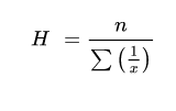
Example 1 - Calculate the harmonic mean of the numbers 13.2, 14.2, 14.8, 15.2 and 16.1
Solution
X | 1/X |
13.2 | 0.0758 |
14.2 | 0.0704 |
14.8 | 0.0676 |
15.2 | 0.0658 |
16.1 | 0.0621 |
Total | 0.3147 |
H.M of X = 5/0.3147 = 15.88
Example 2 - Find the harmonic mean of the following data {8, 9, 6, 11, 10, 5} ?
X | 1/X |
8 | 0.125 |
9 | 0.111 |
6 | 0.167 |
11 | 0.091 |
10 | 0.100 |
5 | 0.200 |
Total | 0.794 |
H.M of X = 6/0.794 = 7.560
For grouped data

Example 3 - Calculate the harmonic mean for the below data
Marks | 30-39 | 40-49 | 50-59 | 60-69 | 70-79 | 80-89 | 90-99 |
F | 2 | 3 | 11 | 20 | 32 | 25 | 7 |
Solution
Marks | X | F | F/X |
30-39 | 34.5 | 2 | 0.0580 |
40-49 | 44.5 | 3 | 0.0674 |
50-59 | 54.4 | 11 | 0.2018 |
60-69 | 64.5 | 20 | 0.3101 |
70-79 | 74.5 | 32 | 0.4295 |
80-89 | 84.5 | 25 | 0.2959 |
90-99 | 94.5 | 7 | 0.0741 |
Total |
| 100 | 1.4368 |
HM = 100/1.4368 = 69.59
Example 4 – find the harmonic mean of the given class
Ages | 4 | 5 | 6 | 7 |
No. Of students | 6 | 4 | 10 | 9 |
Solution
X | F | f/x |
4 | 6 | 1.50 |
5 | 4 | 0.80 |
6 | 10 | 1.67 |
7 | 9 | 1.29 |
| 29.00 | 5.25 |
HM = 29/5.25 = 5.5
Example 5 – calculate harmonic mean
Class | Frequency |
2-4 | 3 |
4-6 | 4 |
6-8 | 2 |
8-10 | 1 |
Solution
Class | Frequency | x | f/x |
2-4 | 3 | 3 | 1 |
4-6 | 4 | 5 | 0.8 |
6-8 | 2 | 7 | 0.28 |
8-10 | 1 | 9 | 0.11 |
| 10 |
| 2.19 |
Harmonic mean = 10/2.19 = 4.55
2.2.6 Quadratic Mean:
The quadratic mean is also called as root mean square. It measures the absolute magnitude of a set of numbers, and is calculated by:
- Squaring each number,
- Finding the mean of these squares,
- Taking the square root of that average.
Formula
The quadratic mean is equal to the square root of the mean of the squared values. The formula is:


Example 1 - Find the Root Mean Square of 2, 4, 9, 10,and 12.
Solution
N= 5
Square all of the numbers. 22,42,92,102, 122 = 4, 16, 81, 100, 144.
= 4 + 16 + 81 + 100 + 144 = 345.
= 345/5 = 69.
= √(69) = 8.31.
Example 2 - Find the Root Mean Square of 3, 6, 2, 9, 1, 7, 2
Solution
N= 6

Example 3 - find the Root Mean Square of -2,-1,-3,1,5.
Solution
N- 5
Square all the values. 4,1,9,1,25
= 4+1+9+1+25/5 = 40/5 = 8
= sqrt(8) = 2.83
Example 4 – find the root mean square of 2, 4, 6, 8, 10, 12
Solution
N- 6
= Square all the values. 4, 16, 36, 64, 100, 144
= 4+16+36+64+100+144/6 = 364/6 = 60.67
= sqrt(60.67) = 7.78
Examples 5- Calculate the root mean square of the following observations; 5, 4, 8, 1 ?
Solution
N= 4
Square all the values. 25, 16, 64, 1
= 25+16+64+1/4 = 106/4 = 26.5
= sqrt(26.5) = 5.14
2.2.7 Moving Average:
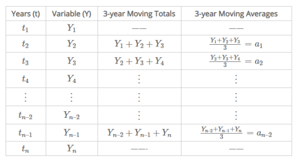
A moving average is a technique to get an overall idea of the trends in a data set; it is an average of any subset of numbers. The moving average is extremely useful for forecasting long-term trends. For any given period, you can calculate a five-year moving average, a four-year moving average, a three-year moving average and so on.
Suppose for a given time period calculate 3 years moving average
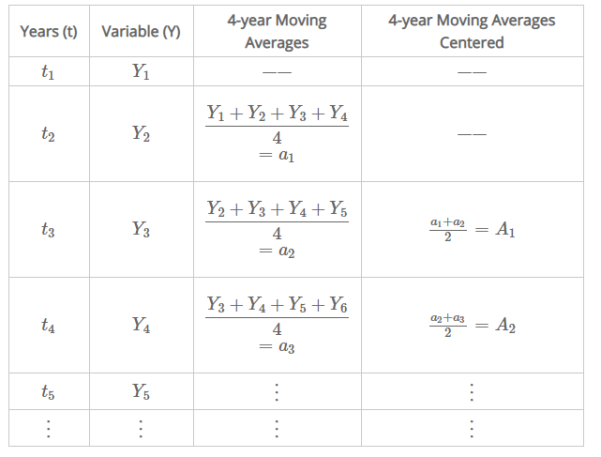
Four year moving average
Example
Compute 5-year, 7-year and 9-year moving averages for the following data.
Year | 1990 | 1991 | 1992 | 1993 | 1994 | 1995 | 1996 | 1997 | 1998 | 1999 | 2000 |
Values | 2 | 4 | 6 | 8 | 10 | 12 | 14 | 16 | 18 | 20 | 22 |
Solution
|
| 5-Year Moving | 7-Year Moving | 9-Year Moving | |||
Years | Values | Total | Average | Total | Average | Total | Average |
1990 | 2 |
|
|
|
|
|
|
1991 | 4 |
|
|
|
|
|
|
1992 | 6 | 30 | 6 |
|
|
|
|
1993 | 8 | 40 | 8 | 56 | 8 |
|
|
1994 | 10 | 50 | 10 | 70 | 10 | 90 | 10 |
1995 | 12 | 60 | 12 | 84 | 12 | 108 | 12 |
1996 | 14 | 70 | 14 | 98 | 14 | 126 | 14 |
1997 | 16 | 80 | 16 | 112 | 16 |
|
|
1998 | 18 | 90 | 18 |
|
|
|
|
1999 | 20 |
|
|
|
|
|
|
2000 | 22 |
|
|
|
|
|
|
Example 2 - Compute 4-year moving averages centered for the following time series:
Year | 1990 | 1991 | 1992 | 1993 | 1994 | 1995 | 1996 |
|
Values | 80 | 90 | 92 | 83 | 87 | 96 | 100 | |
Solution
|
| 4-Year Moving |
| ||
Years | Values | Total | Average | 2 valus moving total | 4 year moving average centered |
1990 | 80 |
|
|
|
|
1991 | 90 | 345 | 86.25 |
|
|
1992 | 92 | 352 | 88 | 174.25 | 87.125 |
1993 | 83 | 358 | 89.5 | 177.5 | 88.75 |
1994 | 87 | 366 | 91.5 | 181 | 90.5 |
1995 | 96 | 393 | 98.25 | 189.75 | 94.875 |
1996 | 100 |
|
|
|
|
1997 | 110 |
|
|
|
|
2.2.8 Progressive Average:
Progressive average is same like moving average as given above
Mean
Mean is the result of combining all the values and dividing the total by the amount of values, given a set of values.
Median
Median is the middle value among the observed set of values and is calculated by arranging the values in ascending order or in descending order and then choosing the middle value.
Mode
Mode is the number from a data set which has the highest frequency and is calculated by counting the number of times each data value occurs.
Empirical relationship between mean, median, mode
The relationship between mean, median and mode can be expressed using Karl Pearson’s formula
(mean – median) = 1/3 (mean – mode)
3(mean – median) = (mean – mode)
Mode = mean – 3(mean – median)
Mode = 3 median – 2 mean
Mean median mode relation with frequency distribution
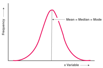
- Frequency Distribution with Symmetrical Frequency Curve
Median, and mode will be equal, if a frequency distribution graph has a symmetrical frequency curve mean
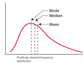
- For Positively Skewed Frequency Distribution
The mean is always greater than median and the median is always greater than the mode, in case of a positively skewed frequency distribution,
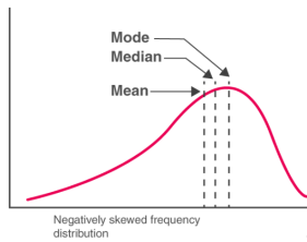
- For Negatively Skewed Frequency Distribution
The mean is always lesser than median and the median is always lesser than the mode, in case of a negatively skewed frequency distribution.
Example 1
The median is 20 and the mean is 22.5. Using these values, find the approximate value of the mode.
Solution:
Given,
Mean = 22.5
Median = 20
Mode = x
Now, using the relationship between mean mode and median we get,
(Mean – Mode) = 3 (Mean – Median)
So,
∴ x = 15
So, Mode = 15.
Example 2
For a moderately skewed distribution mode = 50, mean = 45, find median?
Mean – mode = 3 (mean – median)
45 – 50 = 3(45 – median )
-5/3 = 45 – median
-1.66 = 45 – median
Median = 45 + 1.66 = 46.66 (negatively skewed to left)
Example 3
The mean and median of a moderately skewed distribution are 42.2 and 41.9 respectively. Find mode of the distribution.
Mean – mode = 3 (mean – median)
Mode = 42.2 – 0.9 = 41.3
Example 4
For a moderately skewed distribution, the median price of men's shoes is Rs 380 and modal price is Rs 350. Calculate mean price of shoes.
Mode = 3 median – 2 mean
350 = 3*380 – 2 mean
350 = 1140 – 2mean
Mean = (1140 – 350)/ 2
Mean = 395