Unit -II
Macro analysis of consumer behavior
State economics and policies are directly related to economic welfare and therefore have a significant impact on consumer demand. It has been ignored until now, but it can be used to briefly explain fluctuations in consumption patterns such as consumer goods and help in planning business strategies.
Microeconomic volatility, one of the most important indicators of business, has been rarely studied in India (Garda & Ziemann, 2014). Microeconomic volatility is directly related to economic welfare, as reflected in fluctuations in household economic conditions. Still, it remains an untouched issue by research aimed at understanding the Indian consumer market.
Macroeconomic conditions may be related to household income distribution. This article provides an analysis of motorcycle demand and its relevance in the three states of Maharashtra, Tamil Nadu (TN) and Uttar Pradesh (UP). The states were selected on the premise that Maharashtra and Tennessee are the two top economic performers in the country. Both UP and Maharashtra are larger in terms of population and size compared to Tennessee. And in UP and Maharashtra, the contrast between rural and urban areas and regional inequality are more pronounced compared to Tennessee.
This analysis is collected from employment data from Nielsen's Market Skyline, Nielsen's own database created by the Indian Automobile Manufacturers Association (SIAM), National Accounts Statistics, and Nielsen's Micromarketing and Economics (MME) team database. Secondary data was used. It aims to:
Understand motorcycle sales patterns and changes from 2001 to 2014.
As shown in the 2001 National Accounts Statistics, the state's Gross Domestic Product (SGDP) data is analyzed component by component to identify key sectors and changes that have occurred over the years. These are captured by the sector's share of the total GDP of the three states.
Understand state employment scenarios from 2001 to 2013 and identify changes that have occurred in correlation with state GDP.
To understand the volatility of household income, understand the distribution of households across income groups and their changes over time.
Motorcycle sales
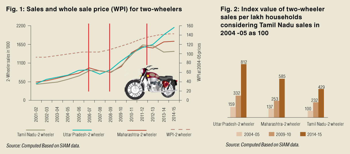
We used motorcycle sales data over the last 15 years to understand demand and analyze consumer behavior patterns. Figure 1 shows that motorcycle sales patterns and price trends are now recognizable. Prices are expressed in the Wholesale Price Index (WPI) for the entire motorcycle industry. The correlation between WPI and state sales data shows that prices did not have a significant impact on sales.
You can also see the clear phases of motorcycle demand in the selected states. The entire period considered here can be divided into four phases:
Phase 1: From 2001-02 to 2006-07, total sales in Maharashtra and UP were about the same. TN followed the same growth trajectory, but sales were lower than in the other two states.
Phase 2: Can be clearly marked between 2006-07 and 2008-09. Before the global recession and during the global recession. In both Maharashtra and UP, sales declined significantly during this period, but TN sales were about the same.
Phase 3: Sales improved significantly during this phase from 2008-09 to 2011-12. Later in this phase, sales in all three states were about the same.
Phase 4: Dramatic changes have been seen since 2011-12. UP showed tremendous growth in motorcycle sales, but Maharashtra maintained slow growth. In contrast, Tennessee sales fell sharply. Given that Tennessee is one of the most economically performing states in the country, this is an unexplained phenomenon.
To handle population factors in the analysis, Figure 2 shows an index of sales per household of Rs 10,000 in all three states 2004-05, 2009-10, and 2014-15. The graph shows that motorcycle sales are far behind the other two states in terms of household perspective.
The industrial and service sectors together contribute more than 94% to TN's total GDP. This is just under 93% of Maharashtra's GDP and about 77% of UP's total GDP.
Services are arguably the most important sector for all three states. From 2011 to 2004, UP achieved much higher growth in the services sector compared to Maharashtra and Tennessee. The construction sector has increased significantly in the last few years, but the overall slowdown in the manufacturing sector has significantly reduced the overall share of the industrial sector in UP. In Maharashtra, the overall share of the industrial sector has fluctuated due to the continuous decline in manufacturing since 2006-07. However, the share of the construction sector has increased significantly. In Tennessee, the manufacturing share has declined since 2011. However, that is just one perspective. For example, shares tend to change as GDP fluctuates by sector. The amount of income generated is more important than the change in stocks.
Change of employment scenario
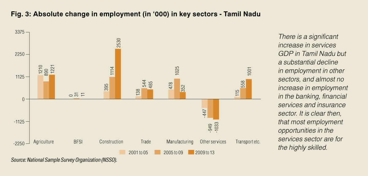
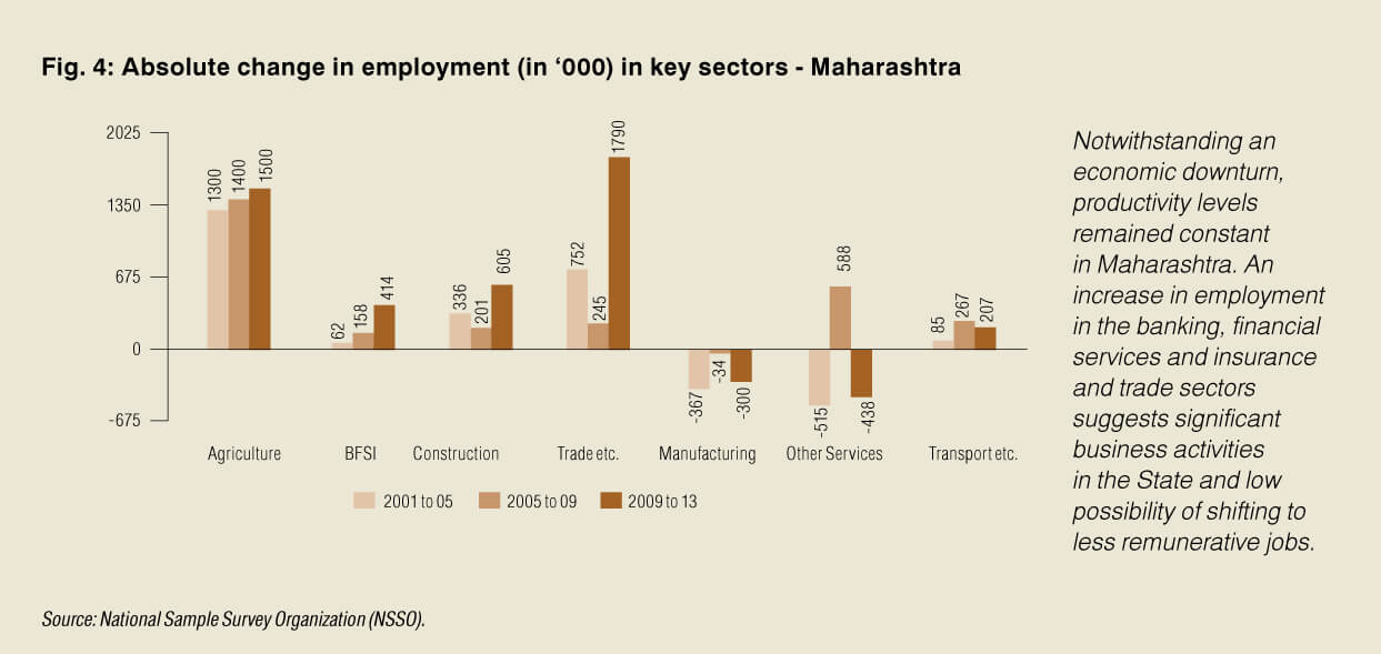
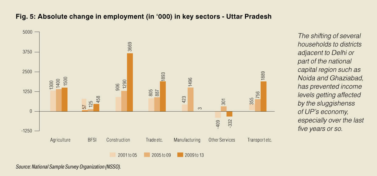
Employment scenarios are one of the best criteria for measuring the economy. However, the changes you experience may be immediate. Still, it clearly shows economic movements and their correlations. Figures 3, 4, and 5 show the percentage of employment in major sectors at four points in time. Absolute changes in each sector provide each state with some interesting contrasting characteristics. The most important ones related to the observed car sales are:
At TN, employment in the construction sector from 2009 to 2013 exceeded Rs 250,000. Employment in the transportation, storage and telecommunications sectors was Rs 100,000. In 2013, the manufacturing industry saw an increase of about 35,000 compared to 2009. Another important point is that in the banking, financial services and insurance (BFSI) sectors, the actual increase in employment in 2009-13 was modest. 11,000 compared to 31,000 in 2005-09.
In Maharashtra, employment growth in the trade, hotel and restaurant sectors was around Rs 180,000 between 2009 and 2013. In the construction sector, the same is about 60,000 rupees. In the manufacturing industry, employment decreased by 30,000 rupees from 2009 to 2013. The BFSI sector saw an increase of more than 400,000, compared to just 11,000 in Tennessee in 2009-13.
UP saw significant changes in employment in the transport and trade sectors, with the exception of the construction sector, from 2009 to 2013. One of the most important points to note is the increase in employment of more than Rs 45,000 in the BFSI sector during this period. There is a major transition from UP, especially to Noida, Ghaziabad and Meerut. This large population, living in UP and working in Metro Manila (NCR), creates a discrepancy between the economy, employment, and demand for goods.
From all of this, we can identify some important issues that can help us understand microeconomic volatility from the right perspective:
In Tennessee, GDP for services has increased significantly, but employment in other sectors has declined significantly, with little increase in employment in the BFSI sector. Therefore, it is clear that most employment opportunities in the service sector are for highly skilled people.
TN's manufacturing GDP has declined significantly, but manufacturing employment has increased. This is only possible if jobs are created at a level below unskilled.
The increase in employment in the construction sector far outweighs the increase in GDP in this sector. This is because the construction sector is labor-intensive and the workforce is primarily composed of low-level or low-paying, unskilled workers.
Tennessee's economic situation has caused a low level of job growth over the last four to five years. This can change the previous income distribution scenario.
In the case of Maharashtra, productivity levels remained constant despite the recession. Increased employment in the BFSI and trade sectors suggests that it is unlikely to shift to significant business activities in the state and less paid jobs.
UP will prevent the population from being adversely affected by the lack of momentum in GDP growth due to increased GDP in the services sector, reduced reliance on manufacturing, and significant increases in employment in the trade, transportation and BFSI sectors. I will.
The relocation of several households to areas adjacent to Delhi or to parts of NCR such as Noida and Ghaziabad has prevented the impact of UP's economy on income levels, especially for the past five years.
Changes in income distribution patterns
Market Skyline 2014-15 is used for this analysis. Household distribution data is available for three years, so 2004-05, 2009-10, 2014-15 have databases for all three states to understand changes in household income distribution at list prices in 2014-1015. It was created. When estimating household distribution across income groups, the consumer price index was examined separately for urban and rural areas.
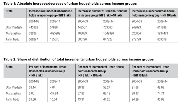
The 2014-15 price considered the household distribution of three income groups, namely those with an annual income of less than 3 rupees, an annual income of 3 to 10 rupees and an annual income of more than 10 rupees. The purpose is to determine which groups are most likely to buy a motorcycle. Discussions with industry insiders suggest that households with incomes of Rs 3 to Rs 10 are most likely to choose motorcycles in terms of affordability.
Table 1 shows the actual changes in the number of households in each of these income groups over the period 2004-2009 and 2009-14 to show how the income distribution changed over time. I am. Tables 1 and 2 clearly show that Tennessee had the lowest number of households in the low-income group, less than 3 rupees per year, when compared between 2004-09 and 2009-05. Therefore, the segment tends to buy motorcycles and is the least growing in Tennessee compared to the other two states. However, the increase in high-income households in Tennessee was about the same as UP, although it was higher in Maharashtra.
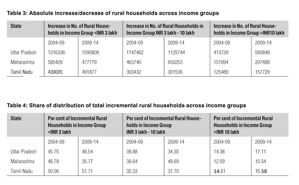
This is even more apparent when looking at the proportion of incremental households in the three income groups. The total growth of middle-income households was the lowest in Tennessee, meaning that the gradual transition of households from low-income to high-income households was the least experienced in urban areas of Tennessee. Tables 3 and 4 show similar trends in rural Tennessee.
Therefore, in both rural and urban TNs, the number of middle-income households has not increased enough to promote the sale of some products, including motorcycles, compared to UP and Maharashtra. Did. Therefore, microeconomic volatility, or instability in income distribution between income groups, is an important factor in explaining the decline in Tennessee motorcycle sales compared to other states.
Note at the end
Household income distribution data for the entire income group on a real basis suggests that TN has experienced higher levels of inequality in its income distribution over the past five years compared to Maharashtra and UP states. This is reflected in household consumption behavior and motorcycle sales. Therefore, studying household income distribution scenarios to predict consumption patterns can facilitate better business planning and strategies in different parts of the country.
Income consumption relationship
The Relationship between Income & Expenditure
The relationship between income and expenses is often referred to as the consumption schedule. It is used to explain the economic trends of the household sector. More goods are bought by consumers when there is an expectation of more money and income. Meaningful money is sometimes spent on spending, even if you don't have enough income to cover them. This is a general economic principle used to explain spending trends in the domestic and global economies. Companies need to extract data on buyer trends within the industry, taking into account the relationship between consumption and savings.
Consumption schedule: Expenditure and income
Consumers buy more products because their disposable income increases as their income increases. As a result, consumption of major purchases and non-essential items increases. Increased consumer spending is not directly related to income. For every $ 1 you earn, your disposable income can cost a small amount. In low-income areas, you may actually spend more than you actually earn at different times.
The difference between income and consumption is the amount of money left over as savings at the end of the month. There are many factors that determine why consumers choose to spend more on products they don't need for their daily living expenses. These include stock market trends, tax law, and even consumer optimism. Economic experts look at historical data and predict future trends based on new market conditions.
Impact of consumer confidence
Consumers do not spend money unless they are confident in their financial situation and strength. This means that consumers are happy to have and maintain a job with the potential for promotion. Wage increases, stock portfolio increases, and tax cuts allow you to put more money in each person's pocket. The combination of these conditions will increase consumer confidence.
Consumer trust is the trust that a buyer can buy now or in the near future. For example, consumer confidence is indicated by the tendency of homebuyers. This is a major purchase that will take decades to pay off. The buyer needs to be not only satisfied with the economy, but also reassured about his personal financial situation in order to make such a large purchase.
Establishing business inventory practices
Another factor affecting consumer confidence in inventory. Supply and demand have a big impact on whether buyers feel they need to buy now. Going back to the home buying example, if there are few homes for sale and interest rates are low, supply will decrease, but demand may increase. While this allows us to make the best possible deals, it can lead to higher purchasing desires among consumers seeking to enter.
Companies need to consider their inventory levels when reviewing consumption schedules and consumer confidence. If any item is in stock, you are less urgent to buy it. Increasing inventories in sectors such as the automotive industry reduce consumer confidence, suggesting that conditions drive savings over spending. Companies in this sector need to pay attention to inventory levels, make inventory levels easier to manage, and avoid staying in inventory for extended periods of time.
No company can manage consumer trust, but it can take proactive steps to protect itself in response to changing buyer trends. Companies may need to increase or decrease manufacturing and wholesale orders. We may also offer promotional prices to maintain profitability and inventory movement. There is a negative relationship between income and spending Low consumer confidence means spending time watching movies, buying new cars and homes, and spending a little extra when you feel your pockets are a little deeper. It means that there are fewer people to do it.
Absolute, Relative and Permanent Income Hypothesis (With Diagram)
Absolute Income Hypothesis:
Keynes's consumption function has become known as the "absolute income hypothesis" or theory. His statement on the relationship between income and consumption was based on "basic psychology." He said consumption is a stable function of current income (more specifically, current disposable income, or post-tax income).
By operating the "Psychological Law", his consumption function is 0 <MPC <1 and MPC <APC. Therefore, Keynes's absolute income hypothesis has a non-proportional relationship between consumption and income (that is, APC> MPC). His consumption function can now be rewritten in the following format
C = a + bY, where a> 0 and 0 <b <1.
It may be added that all the characteristics of Keynes's consumption function are based on "basic psychological laws", that is, experience and intuition, rather than empirical observations.
(I) Consumption function in the light of empirical observation:
Meanwhile, in the late 1930s and early 1940s, experience-oriented economists attempted to test the conclusions made by Keynes's consumption function.
(II) Short-term budget data and circular data:
First, consider the budget survey data or cross-section data for the cross section of the population, and then consider the time series data. The first set of evidence came from the 1935-36 and 1941-42 budget surveys. These budget surveys seemed to be in line with Keynes' own conclusions about the relationship between consumption and income. US time series data from 1929-44 also provided fairly good support for Keynes's theoretical consumption function.
This empirical consumption function, derived from the 1929-44 time series data, is sometimes referred to as the "circular" consumption function because the period of interest is not long enough. Anyway, we can conclude that these two datasets that generated the consumption function are in agreement with Keynes's consumption equation C = a + bY.
In addition, 0 <b <1 and AMC <APC.
- Long-term time series data
However, Simon Kuznets, winner of the 1971 Nobel Prize in Economic Sciences, considered the long period from 1869 to 1929. His data can be described as long-term or long-term time series data. This data showed that there was no long-term change in consumption, despite a very large increase in income during the period. Therefore, the long-term historical data that generated the long-term or long-term consumption function did not match the Keynesian consumption function.
Here's what we get from Kuznets' data:
(A) There is no autonomous consumption. That is, with the "a" term of the consumption function
(B) Proportional long-term consumption function with no difference between APC and MPC. In other words, the equation for the long-term consumption function is C = bY.
Since a = 0, the long-term consumption function is such that APC does not change over time and MPC = APC is all income levels, in contrast to the relationship between short-term non-proportional (MPC <APC) consumption and income. It is a function that occurs in. Because it is proportional, the long-term consumption function starts at the origin and the non-proportional short-term consumption function starts at a point above the origin. In fact, Keynes was interested in the long-term situation.
However, it is confusing and confusing to us that empirical studies suggest two different consumption functions, the non-proportional cross-section function and the proportional long-term time series function.
2. Relative income hypothesis:
Consumption studies were then directed to resolve obvious conflicts and contradictions between Keynes's absolute income hypothesis and observations by Simon Kuznets. Previous hypotheses have stated that MPC <APC in the short term, but Kuznets' observations indicate that MPC = APC in the long term.
One of the early attempts to provide a resolution of the conflict between the short-term consumption function and the long-term consumption function). It was S's "relative income hypothesis" (R1H). Duesenberry in 1949. Duesenberry believed that the basic consumption function was long-term and proportional. That is, the average percentage of income consumed does not change in the long run, but there can be fluctuations between consumption and income in short-term cycles.
Duesenberry's RIH is based on two hypotheses. The first is the relative income hypothesis, and the second is the past peak income hypothesis.
Duesenberry's first hypothesis is that consumption depends not on "absolute" levels of income, but on "relative" income, that is, income relative to the income of the society in which the individual lives. This is because their relative position in the family income distribution influences individual consumption decisions.
Household consumption is determined by the income and spending patterns of neighbors. They tend to imitate or imitate the consumption standards maintained by their neighbors. Specifically, relatively low-income people try to "catch up with Jones." They consume more and save less. This mimicking or mimicking nature of consumption is described by Duesenberry as a "demonstration effect."
The result of this hypothesis is that an individual's APC depends on his relative position in income distribution. Relatively high-income families experience low APCs, and relatively low-income families experience high APCs. On the other hand, if the income distribution is relatively constant (that is, the relative position of each family remains unchanged while the income of all families is increasing). After that, Dusenbury claims that APC remains the same.
Therefore, in total, there is a proportional relationship between total income and total consumption. Note MPC = APC. Therefore, R1H states that there is no apparent discrepancy between the results of the cross-budget survey and the long-term aggregated time series data.
From the perspective of the second hypothesis, we can explain the short-term periodic behavior of Dusenbury's total consumption function. Duesenberry hypothesized that the family's current consumption is affected not only by their current income, but also by their past peak income levels. That is, C = f (Yri, Ypi). Where Yri is the relative income and Ypi is the peak income.
This hypothesis states that family spending is primarily motivated by habitual behavioral patterns. As current income increases, households tend to consume more, but slowly. This is because habitual consumption patterns are relatively low and people slowly adjust the consumption standards established by previous peak incomes to current rising income levels.
On the other hand, if current income declines, these households will find it difficult to reduce the consumption established by previous peak income, so they will not reduce consumption immediately. Therefore, during a recession, consumption increases as part of income, and during prosperity, consumption slowly increases as part of income. Therefore, this hypothesis produces a non-proportional consumption function.
Duesenberry describes the short-term and long-term consumption functions, and finally, the adjustment between these two types of consumption functions can be shown in Figure 3.39. The cyclical rise and fall of income levels creates an asymmetric consumption-income relationship labeled CSR. In the long run, smoothing these fluctuations in income levels will result in a proportional consumption-income relationship labeled the CLR.
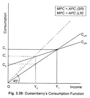
As national income increases, consumption increases along with long-term consumption, the CLR. Please note that the total consumption of OY0 on income is OC0. When income increases to OY1, consumption increases to OC1. This means a constant APC as a result of the steady growth of national income.
Now suppose that a recession occurs, leading to a previously achieved peak income of OY1 and a decline in income levels to OY0. Duesenberry's second hypothesis has been put into practice. Households maintain previous consumption levels that they enjoyed at past peak income levels. In other words, hesitate to lower consumption standards in line with the CLR. Consumption does not decrease to OC0, but decreases to OC'1 (> OC0) with income OY0. At this income level, APC is higher and MPC is lower than for OY1.
If income rises as a result of an economic recovery, consumption will rise in line with CSR as people seek to maintain customary or customary consumption standards affected by previous peak incomes. When you reach OY1 level income, consumption moves along the CLR. Therefore, short-term consumption is affected by what Dusenberry called the "ratchet effect." It rises as income levels rise, but does not fall as income declines.
3. Permanent Income Hypothesis:
Another attempt to reconcile three sets of clearly contradictory data (cross-section or budget survey data, periodic or short-term time-series data, and Kuznets long-term time-series data) won the Nobel Prize in 1957. Performed by economist Milton Friedman. .. Like Duesenberry's RIH, Friedman's hypothesis believes that the basic relationship between consumption and income is proportional.
However, according to Friedman, consumption does not depend on "absolute" or "relative" income, but on "permanent" income based on expected future income. Therefore, he finds a relationship between consumption and permanent income. His hypothesis is then explained as the "Permanent Income Hypothesis" (PIH). PIH shows the relationship between constant consumption and constant income.
Friedman divides the currently measured income (that is, the income actually received) into two parts: permanent income (Yp) and temporary income (Yt). Therefore, Y = Yp + Yt. Permanent income can be considered as "average income". This depends on the income you expect or expect to receive over the long term. Temporary income, on the other hand, consists of an unexpected, unexpected, or plunge increase or decrease in income (for example, income received from a lottery ticket or race). Similarly, he distinguishes between permanent consumption (Cp) and transistor consumption (Ct). Temporary consumption may be considered unexpected spending (such as unexpected illness). Therefore, the measured consumption is the sum of the permanent and temporary elements of consumption. That is, C = Cp + Ct.
Friedman's basic argument is that constant consumption depends on constant income. The basic relationship of PIH is that constant consumption is proportional to constant income, which indicates a fairly constant APC. That is, C = kYp. Where k is a constant, equal to APC and MPC.
While reaching the above conclusions, Friedman assumes that there is no correlation between Yp and Yt, between Yt and Ct, and between Cp and Ct. That is
RYt. Yp = RYt. Ct = RCt. Cp = 0.
High (or low) permanent income does not correlate with high (or low) temporary income because Yt is not corrected by Yp. For the entire group of households in all income groups, the temporary income (both positive and negative) offsets each, so the average temporary income is equal to zero. This also applies to the temporary element of consumption. Therefore, when all families are combined, the average temporary income and average temporary consumption are zero.
Yt = Ct = 0 where Y and C are averages. Now it continues
Y = Yp and C = Cp
Consider some families with above-average measured income, rather than the average of all families. This happens because these families enjoyed unexpected income, which resulted in a positive temporary income and Yp <Y.
We are now in a position to resolve the obvious contradictions between cross-sectional area and long-term time series data, and to show a stable and constant relationship between constant consumption and constant income.
The line Cp = kYp in Figure 3.40 shows the proportional relationship between constant consumption and constant income. This line cuts the CSR line at point L, which corresponds to the average measured revenue of the population with Yt = 0. This average measurement revenue produces an average measurement and a durable Cp.
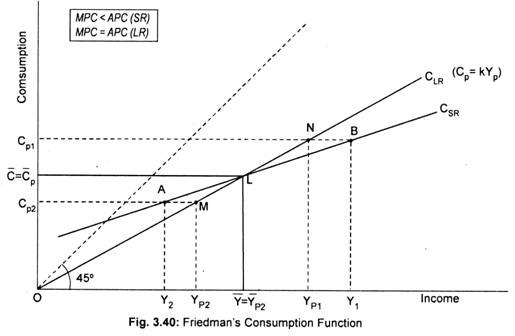
First, consider a sample group of populations whose average income is above the average of the population. For this population group, transistor revenues are positive. The horizontal difference between the short-term consumption function and the long-term consumption function (points N and B and points M and A) represents temporary income. The measured income is equal to the permanent income at the intersection of these two consumption functions, that is, the point L in the figure where the temporary income is zero.
In the case of the sample group whose average income exceeds the national average measured income (Y1), it exceeds the permanent income (YP1). At the (CP1) level of consumption (ie, point B), the average measured income for this sample group exceeds the permanent income YP1. Therefore, this group currently has a positive average temporary income.
Next, consider another sample group of populations whose average measured income is below the national average. In this sample group, the temporary income component is negative. At Cp2 level consumption (that is, point A on the CSR), the average measured income is below the permanent income Yp2. Now, if you combine points A and B, you get a section consumption function labeled CSR. This consumption function provides an MPC with a value smaller than the long-term proportional consumption function Cp = kYp. Therefore, in the short term, Friedman's hypothesis produces a consumption function similar to Keynes's hypothesis, MPC <APC.
But over time, as the economy grows, the temporary factor diminishes to zero throughout society. Therefore, the measured consumption and measured income values are constant consumption and constant income. Combining points M, L, and N yields a long-term proportional consumption function that correlates constant consumption with constant income. In this line, the APC is fairly constant. That is, APC = MPC
In ordinary terms, investing means buying stocks, stocks, bonds, and securities that are already on the stock exchange. However, this is often not a true investment, because it is just a transfer of existing assets.
Importance:
The level of income, output and employment within the economy depends on effective demand, which depends on spending on consumer and investment goods (Y = C + I).
The propensity to consume depends, as we've learned, on the propensity to consume, which is more or less stable during a short period of your time and is a smaller amount than one. Therefore, it must be more hooked in to other components of income (investment).
Of the 2 components of income (consumption and investment), consumption is stable and fluctuations in effective demand (income) are tracked through fluctuations in investment. Therefore, investment will play a strategic role in determining the extent of income, output and employment at just one occasion .
You can also establish the importance of investing in other ways. So as to take care of an income equilibrium level (Y = C + I), the sum of consumer spending and investment spending must be adequate to total income (Y). However, consistent with the psychological law of consumption given by Keynes, as income increases, so does consumption, but but income. This suggests that a number of your income growth are going to be saved instead of used.
Savings must be invested to bridge the gap between increased income and increased consumption. If this gap isn't filled by increased investment spending, the result are going to be an unintended increase in inventories of commodities (inventory), which successively will cause depression and mass unemployment. Therefore, investment dominates the roost. In Keynesian economics, investment means actual investment. That is, an investment in building other sorts of productive capital stock within the community, including new machinery, new factory buildings, roads, bridges, and increased inventories.
This doesn't include the acquisition of existing stock, stock or securities. These are just exchanges of cash from one person to a different . Such investments are merely financial investments and don't affect employment levels within the economy. An investment may be a flow variable, and therefore the corresponding one may be a stock variable called capital.
Type of investment:
The investment is often a personal investment or a public investment and may be guided or autonomous. Induced investment is an investment that changes as income changes, which is why it's called income elasticity. During a free corporate capitalism , investment is driven by profit motives. Such investments are very sensitive to changes in income. That is, the more income you've got , the more investment you've got triggered. Therefore, the form of the induced investment curve is sloping upwards, indicating that investment is increasing as a results of increased income.
According to Hicks, there are two sorts of investments, one that's triggered as described above and one that's autonomous, and is independent of output fluctuations. . They will be considered autonomous investments. I will. "
Autonomous investment isn't sensitive to changes in income. In other words, it's nothing to try to to with changes in income and isn't guided or triggered solely by profit motives. Autonomous investments are made primarily by the govt and aren't supported profit considerations.
Autonomous investment may be a hallmark of war and planned economies, and is usually mentioned as autonomous investment because, for instance , spending on weapons and equipment to strengthen India's defenses occurs no matter income or profit level. Professor Hansen argued that autonomous investment is usually related to factors like new production technologies, product introductions, new resource development, and increase .
Induced investments are specially made to get large volumes. The curve of autonomous investment extends from left to right and is represented by a line parallel to the horizontal income axis.
Total investment and net investment:
As we have seen, investments of the nature of spending on fixed capital goods over a period of time, or of the additional nature of raw materials and unsold consumer goods inventories, are called gross investments. However, investment substitution means the expenditure incurred to keep the stock of capital intact in the economy. This type of spending is made to offset the depreciation, wear and tear of existing capacity. Therefore, net investment is an excess of total investment that exceeds alternative investment. Therefore, the term net investment may also be used for capital formation.
Symbolically:
Ig = In + Ir
Where Ig is total investment, net investment and, in Ir, alternative investment, also known as capital depletion. It is the In fluctuation that causes the Y, O, and E fluctuations, both short-term and long-term. During the period Ig> Ir, In is positive, which means that the stock of capital is increasing equally to In, which leads to an increase in production capacity. If Ir> Ig, In is negative, which can reduce the stock of capital and adversely affect production capacity. However, if Ig = Ir, then In = O, which means that the economy is improving its capacity loss due to obsolescence and depreciation.
It goes without saying that net investment may include spending on new durable goods in addition to spending on new capital goods. Therefore, in a sense, it would be more appropriate to define net investment as a net addition to capital stock, including producers and durable goods. Capital here means the accumulation of inventories of plants and equipment held by the business unit. Therefore, it is clear that for economic growth, that is, if the economy grows over time, its capital stock must also grow.
Investment determinants:
Private investment (induced investment) depends on the marginal efficiency of capital and interest rates. The marginal efficiency of capital, in turn, depends on volatile future expectations. Therefore, private investment can be very capricious and very low, but in reality it should be very high.
Future entrepreneurs will continue to compare marginal efficiency of capital with interest rates and decide to invest only if the former is higher than the latter. If the interest rate is higher than MEC, there is no investment. (In other words, if profit expectations are not very bright); that's why investment falls to low levels during the recession, despite all sorts of encouragement to invest more in retail investors. Is.
Classical economists considered investment dependent on interest rates. For them, this was an important means of regulating investment in the system. This is why they are overly dependent on interest rates to control fluctuations. They always believed that manipulating interest rates could restore the stability of the economic system. Until the Great Depression of the 1930s.
Keynes also adhered to this view and believed in the effectiveness of interest rates in solving the problem of periodic fluctuations. But then he realized its weakness and stopped overemphasizing it as a periodic stabilizer. Keynes found that investment depends not on interest rates, but on psychological factors such as marginal efficiency of capital. As a result, I was forced into the background. There is no doubt that marginal efficiency of capital is a major determinant of investment, but since both determine it, the impact of interest rates cannot be ignored.
The important role of public investment, also known as autonomous investment, can be borne by the government to prevent the economy from falling to lower income levels. Due to the nature of the case, public investment has nothing to do with profit motives. Since stable investment is essential for the investment multiplier to have a positive impact on income, output and employment, profits to guide more investment, a function realized only by public investment during a recession. Motivation other than is required. In addition, the amount of public investment can be managed, as well as the investment multiplier can be expanded to the extent that it can function with greater power than other methods.
In addition, the government can prevent it from leaking out of the flow of spending, and it can time it, allowing the multiplier to play completely and freely. There is no reason why public investment should not only create jobs but also wealth, and that its negative effects (if any) cannot be offset as a result of its beneficial effects of the multiplier on personal consumption. Therefore, the importance of public investment. Therefore, it is necessary to analyze various measures that stimulate investment.