UNIT3
PRODUCTION FUNCTION
Isoquant Curves
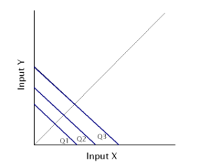
These lines represent various input combinations which produce the same levels of output. The producer can choose any of these combinations available to him because their outputs are always the same. Thus, we can also call them equal product curves or production indifference curves.
Just like indifference curves, isoquants are also negatively-sloping and convex in shape. They never intersect with each other. When there are more curves than one, the curve on the right represents greater output and curves on the left show less output.
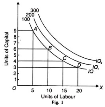
Consider the table below. It shows four combinations, i.e. A, B, C and D, which produce varying levels of output.
Factor combinations | Units of Labour | Units of Capital |
A | 5 | 9 |
B | 10 | 6 |
C | 15 | 4 |
D | 20 | 3 |
Plotting these figures on a graph provides us with this curve (Figure 1):
Source: Economics discussion.net
The X-axis shows units of labour, while the Y-axis represents units of capital. Points A, B, C and D are combinations of factors on which IQ is the level of output, i.e. 100 units. IQ1 and IQ2 represent greater potential output.
Isocost Lines
Isocost lines represent combinations of two factors that can be bought with different outlays. In other words, it shows how we can spend money on two different factors to produce maximum output. These lines are also called budget lines or budget constraint lines.
Let’s assume that a farmer has Rs. 1,000 to spend on labour costs and ploughs for farming. The cost of one such plough and wage per labourer is Rs. 100. Considering his total outlay of Rs. 1,000, he can spend that money in the following combinations:
Ploughs | 0 | 100 | 200 | 300 | 400 | 500 | 600 | 700 | 800 | 900 | 1000 |
Labour | 1000 | 900 | 800 | 700 | 600 | 500 | 400 | 300 | 200 | 100 | 0 |
The farmer, in this case, can either spend the entire sum of Rs. 1,000 on just ploughs by buying 10 of them. Similarly, he can also spend it all on labour by employing 10 labourers. He can even purchase both, labour and ploughs using different combinations as shown above. The total outlay of Rs. 1,000 will remain the same. Hence, the isocost line will remain straight as shown below:
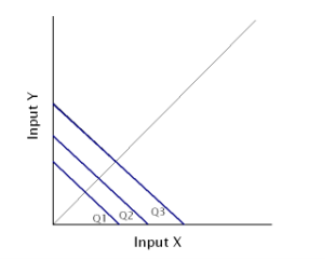
The x-axis represents units of ploughs, and Y-axis would show units of labour. Output levels are shown by a straight line because they remain constant.
Law of Variable Proportions or Returns to a Factor
This law exhibits the short-run production functions in which one factor varies while the others are fixed.
Also, when you obtain extra output on applying an extra unit of the input, then this output is either equal to or less than the output that you obtain from the previous unit.
The Law of Variable Proportions concerns itself with the way the output changes when you increase the number of units of a variable factor. Hence, it refers to the effect of the changing factor-ratio on the output.
In other words, the law exhibits the relationship between the units of a variable factor and the amount of output in the short-term. This is assuming that all other factors are constant. This relationship is also called returns to a variable factor.
The law states that keeping other factors constant, when you increase the variable factor, then the total product initially increases at an increases rate, then increases at a diminishing rate, and eventually starts declining.
Why is it called the Law of Variable Proportions?
As one input varies and all others remain constant, the factor ratio or the factor proportion varies. Let’s look at an example to understand this better:
Let’s say that you have 10 acres of land and 1 unit of labour. Therefore, the land-labour ratio is 10:1. Now, if you keep the land constant but increase the units of labour to 2, the land-labour ratio becomes 5:1.
Therefore, as you can see, the law analyses the effects of a change in the factor ratio on the amount of out and hence called the Law of Variable Proportions.
Law of Variable Proportions Explained
Let’s understand this law with the help of another example:
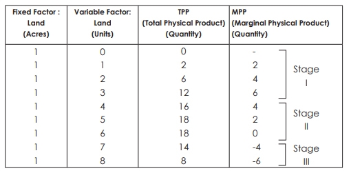
In this example, the land is the fixed factor and labour is the variable factor. The table shows the different amounts of output when you apply different units of labour to one acre of land which needs fixing.
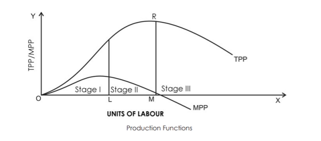
The following diagram explains the law of variable proportions. In order to make a simple presentation, we draw a Total Physical Product (TPP) curve and a Marginal Physical Product (MPP) curve as smooth curves against the variable input (labour).
Three Stages of the Law
The law has three stages as explained below:
Significance of the three stages
Stage I
A producer does not operate in Stage I. In this stage, the marginal product increases with an increase in the variable factor.
Therefore, the producer can employ more units of the variable to efficiently utilize the fixed factors. Hence, the producer would prefer to not stop in Stage I but will try to expand further.
Stage III
Producers do not like to operate in Stage III either. In this stage, there is a decline in total product and the marginal product becomes negative.
In order to increase the output, producers reduce the amount of variable factor. However, in Stage III, he incurs higher costs and also gets lesser revenue thereby getting reduced profits.
Stage II
Any rational producer avoids the first as well as third stages of production. Therefore, producers prefer Stage II – the stage of diminishing returns. This stage is the most relevant stage of operation for a producer according to the law of variable proportions.
Law of Variable Proportions in terms of TPP and MPP
The explanation is as follows:
Law of Variable Proportions – in terms of TPP
We know that the law of variable proportions shows the relationship between units of a variable factor and the total physical product.
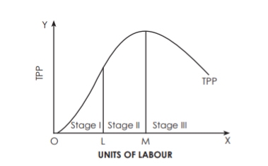
Also, if we keep other factors constant and increase the units of the variable factor, then the TPP initially increases at an increasing rate, then at a diminishing rate, and finally declines. Therefore, it has three clear stages:
Example of Law of Variable Proportion in terms of TPP
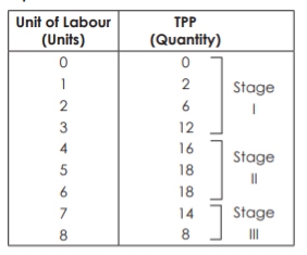
Diagram of Law of Variable Proportion in terms of TPP
Law of Variable Proportions in terms of MPP
The law also states that if we keep all other factors constant and increase the units of a variable factor, then the marginal physical product initially increases, then decreases, and finally becomes negative. Therefore, it has three stages:
Reason for the Operation of the Law
Economic region
Economic region a territorial component of a country’s national economy. Economic region is characterised by specific economic-geographical status, by an economic unity, by distinctive natural and economic conditions, and by a production specialization based on territorial social division of labor. Under capitalism, in the heat of competition economic regions form and develop spontaneously. Under socialism, based on the economic laws of socialism, the territorial division of labor develops, and economic regions form develops in a planned fashion.
In the formation of economic regions, specialization within the social territorial division of labor plays the principal role. The boundaries of a region is determined by the specialised branches action and major auxiliary facilities—the associated cooperative suppliers of raw materials, assemblies, and parts.
Economic region is also influenced by natural conditions such as the natural fertility of the soil, and the climate, the presence of large deposits of minerals.
Other factors influencing the economic region formation are administrative and political units , technical and economic conditions.
The three levels of economic regions are as follows: large (macroregions), administrative (mesoregions), and lowest-level (microregions).
Large economic regions comprise three types: Union republics, groups of Union republics, and groups of autonomous republics. The large economy determines territorial proportions of national economies. It also determines the trends in the location of productive forces throughout the national economy.
Administrative economic regions form the basis of the country’s territorial makeup. It includes the basic elements in the territorial planning and management of the national economy.
Lowest-level economic regions are low-level administrative regions that include the primary territorial elements in the classification of economic regions.
Optimum factors of production
Definition
All factors of production can be varied in the long run. The profit maximisation firm will choose the least cost combination factors to produce a given level of output. The least cost combination or the optimum factor combination refers to the combination of factors with which a firm can produce a specific quantity of output at the lowest possible cost.
Optimum factors of production are explained in two methods are as follows
Formula:
Mppa = Mppb = Mppc = Mppn
Pa Pb Pc Pn
Where as,
a, b, c, n are different factors of production.
Mpp is the marginal physical product.
A firm compares the Mpp / P ratios with that of another. A firm will reduce its cost by using more of those factors with a high Mpp/ P ratios and less of those with a low Mpp / P ratio until they all become equal.
2. The isoquant approach - The least cost combination of-factors is explained with the help of iso-product curves and isocosts. The optimum factors combination or the least cost combination refers to the combination of factors to produce a specific quantity of output at the lowest possible cost. The least cost combination of factors for any level of output when the iso-product curve is tangent to an isocost curve
The choice of a particular combination of factors depends on technical possibilities of production and the prices of factors used for the production of a particular product.
The prices of factors are represented by the iso-cost line. The Iso cost line is very important in determining what combination of factors the firm will choose for production
For ex, a firm has to spend 300/-on the factors of production such as labour and capital. Price of labour is Rs. 4 per labour hour and the price of capital is Rs. 5 per machine hour. With outlay of Rs. 300, a firm can buy 75 units of labour or 60 units capital). In the below figure, OB represent 75 units of labour and OA represent 60 units of capital.
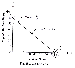
This line AB is called iso-cost line, the combination of various factors which a firm can buy with a constant outlay. The iso-cost line is also called the price line or outlay line.
Assumption of optimum factor combination
The optimum factor combination is explained in the below diagram
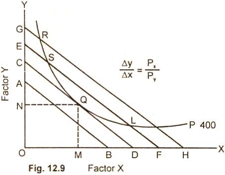
The entrepreneur decides to produce 400units of output which is represented by isoquant P. The 400 unit of output can be produced by any combination of factor X(labour) and Factor Y (capital) such as R, S, Q, L and P lying on the isoquant. For producing 400 units, the cost will be minimum at point Q, which the iso-cost line CD is tangent to the given isoquant. At no other point such as R, S,L, P the cost is minimum. Therefore the firm will not choose any combination of R,S,L,P.
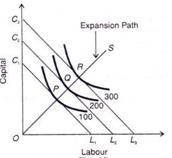
In economics, an expansion path is a line connecting optimal input combinations as the scale of production expands. A producer seeking to produce the most units of a product in the cheapest possible way to increase production along the expansion path.
Definition
Economist Alfred Stonier and Douglas Hague defined expansion path as,” that line which reflects least cost method of producing different levels of output, when factor prices remains constant”.
Assumption
In order to maximise profits, the firm combines labour and capital in such a way that the ratio of their MP is equal to the ratio of their prices

This occurs at a point of tangency between an isocost line and an isoquant curve.
In the above figure, the different isoquant lines areC1L1,C2L2,C3L3. Keeping the prices of factors constant, the different isoquant lines are shown parallel to each other. There are three isoquants ie 100, 200, 300 representing successively higher level of output.
At point P, the firm is at equilibrium, where the isoquant 100 is tangent to its corresponding isoquant line C1L1. Similarly the firm is equilibrium at point Q and R, where the isoquant 200 and 300 is tangent to its corresponding isoquant line C2L2 and C3L3. Each point of tangency implies optimum combination of capital and labour that produces optimum level of output. The line OS joining the equilibrium point P,Q,R from the origin is the expansion path of the firm.
In long run, no factors are fixed. Return of scale refers to proportionate change in productivity from proportionate change in all the inputs.
Definition:
“The term returns to scale refers to the changes in output as all factors change by the same proportion.” Koutsoyiannis
“Returns to scale relates to the behaviour of total output as all inputs are varied and is a long run concept”. Leibhafsky
Types of return of scale
1. Increasing return of scale
2. Constant return of scale
3. Diminishing return of scale
Explanation
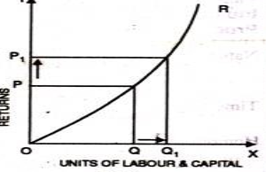
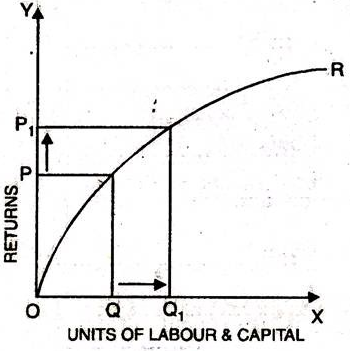
- When proportionate increase in factors of production leads to higher proportionate increase in production refers to increasing return of scale.
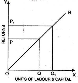
- In the below figure, x axis represent increase in labour and capital while Y axis represent increase in output. When labour and capital increases from Q to Q1, output also increases from P to P1 which is higher than the change in factors of production ie labour and capital
2. Diminishing return of scale

3. Constant return of scale

Economies of scale are the factors which reduces the production cost as the volume of output increases. This means firm produces more output, then marginal cost of production decreases.
Economies of scale is divided into internal and external
Internal economies of scale – internal economies are caused by factors within the firm. It measures the company efficiency of production. The company focus on improving the output to reduce the product average cost.
Six different types of internal economies of scale: (1) technical, (2) managerial, (3) marketing, (4) financial, (5) commercial, and (6) network economies of scale.
2. Managerial economies of scale - the employment of specialised workforce result in managerial economies of scale. As the organisation grow, they hire more expert staff and create a specialised business unit. The firm efficiency is increased by employing specialist, accountants, human resource, etc which will result in reducing the cost of production and increase revenue.
3. Marketing economies of scale – marketing economies of scale is the ability to spread advertising and marketing budget over an increasing output. As the production increases the firm can fix marketing expenses, which will reduce the per unit cost of production. Better advertisement result in reaching larger audience and increase the sale of the firm.
4. Financial economies of scale – access of financial and capital market result in financial economies of scale. Large firms find easier and cheaper to raise funds. As the firm grow, it is considered to be more credit worthy. They can easily raise fund from banks, stock markets.
5. Commercial economies of scale – reduction in price due to discounts or bargaining power result in commercial economies of scale. Larger firms can buy goods and services in larger quantities. Thus they get larger discount and can bargin to negotiate lower prices. This means they pay less for each item purchases.
6. Network economies of scale - when the marginal costs of adding additional customers are extremely low result in network economies of scale. This means larger firm can support large numbers of new customers with their existing infrastructure can substantially increase profitability as they grow.
External economies of scale – external economies of scale are caused by changes outside the firm but within the industry. The factors affect the whole industry. four different types of external economies of scale: (1) infrastructure, (2) supplier, (3) innovation, and (4) lobbying economies of scale.
2. Specialization economies of scale – when suppliers and workers focus on a particular industry due to its size result in specialization economies of scale. When company within the industry increases its size and numbers, suppliers focus in that particular industry. Similarly, similarly workers find job in those industry which is growing in size.
3. Innovation economies of scale – increases public and private research result in innovation economies of scale. Industries have significant impact on the society result in growing public interest. This allows them to collaborate with research facilities and university to improve their products and processes
4. Lobbying economies of scale - Lobbying economies of scale arise from an increase in bargaining power as industries become more significant. The government is ready to compromise as these industry provide a lot of jobs and pay a significant amount of taxes.
Diseconomies of scale – diseconomies of scale occur when firm become too large or inefficient. This happens when average cost per unit start rising.
Diseconomies of scale are divided into two types
- Inefficient management - the lack of efficient or skilled management is the main cause of internal diseconomies. When the firm expand beyond a certain limit, the manager find difficulty in managing and coordinating the process of production efficiently which adversely affect the operational efficiency.
b. Technical difficulties - another cause of internal diseconomies is the emergence of technical difficulties. There is a optimum point of technical economies in every firm. If the firm goes beyond the technical limit then technical diseconomies arises.
c. Production diseconomies – this happens when the expansion of a firm’s production leads to rise in the cost per unit of output. This arises due to use of less efficient factors.
d. Marketing diseconomies – rise in the production cost is accompanies by marketing diseconomies. As the firm grows, advertisement cost increases. It is important to send right message to the target audience.
e. Financial diseconomies – the financial capital cost rises when the scale of production increases beyond the optimum scale. It is due to the more dependence on external finances.
2. External diseconomies – external diseconomies are suffered by the firms operating in a given industry and not by a single firm. Some of the diseconomies are as follows.
b. Diseconomies of strains on infrastructure – localization leads to increase the demand for transportation and therefore transport cost rises. The communication system is also overtaxed in that region. This result in strain on infrastructure and the production cost rises.
c. Diseconomies of high factor prices – competition among the firms affect the factors of production. As a result, the production cost rises. The growth and expansion of an industry will rise the production cost.
An isoquant is oval shaped as shown in the below figure. The firm will produce only in those segments of isoquant which lies between the ridge lines. The ridge lines are the locus of point where factors of marginal products are zero.
The upper ridge lines represent zero MP of capital and the lower ridge line implies zero MP of labour. Inside the ridge lines, production techniques are efficient. While production techniques are inefficient outside the ridge lines.

In the above figure, OA and OB are ridge lines on the oval shaped isoquant and in between the lines are point G,J, L, N,H,K,M,P are unit of capital and labour employed to produce 100, 200, 300 and 400 units of production.
For ex, OT units of labour and ST unit of capital are used to produce 100 units of product. The same 100 units of output can be produced by same quantity of labour OT and less quantity of capital VT. Thus unwise producer will produce outside the ridge lines.
There are various concepts of cost. A firm may use different concepts depending upon a particular situation and the type of business decision to be made. An understanding of these concepts will be helpful to the firm.
A. Money Cost – Implicit and Explicit
Implicit costs (IC) are due to the factors which the entrepreneur himself owns and employs in the firm. In other words they are the imputed value of the entrepreneurs own resources and services. The wage or salary for the services of the entrepreneur, interest on the money capital invested by him and the money rewards for other factors owned and used by him in the firm are known as implicit costs. If these services or factors are sold elsewhere by the entrepreneur he would have earned an income. Thus, implicit costs are the opportunity costs of the factors owned and used by the entrepreneur. Since direct cash payments are not made by them, these costs are called implicit costs. Implicit cost is also called indirect cost.
IC = Imputed cost of resources owned by the entrepreneur
= Opportunity cost of resources owned by the entrepreneur
= Indirect Cost
= Implicit Cost
Explicit costs (EC) are the contractual cash payments made by the firm for purchasing or hiring the various factors. In other words, explicit costs refer to the actual expenditures of the firm to hire, rent, or purchase the inputs its requires in production. They include wages and salaries, payments for raw materials, power, light, fuel, advertisements, transportation and taxes. Explicit money cost is the accounting cost, because an accountant takes into account only the payments and charges made by the firm to the suppliers of various productive factors. Explicit cost also refer to out-of-pocket cost or direct cost.
EC = Expenditure on hiring or purchasing inputs
= Out of pocket cost = Direct cost
B. Accounting Cost and Economic Cost
Accounting cost refers only to the firm’s actual expenditures or explicit costs. Accounting costs are important for financial reporting by the firm and for tax purposes. However, for managerial decision making purposes economic cost is the relevant cost concept.
An economist would include both explicit and implicit costs in the cost of production. Therefore, economic costs equal to explicit costs plus implicit costs. Thus, we can make a distinction between economic cost and accounting cost.
This distinction between explicit and implicit costs is important in analyzing the concept of profit. From the economist’s point of view profit is the difference between total revenue and economic costs. On the other hand, accounting profit, that is, accountant’s concept of profit, is the difference between total revenue and accounting costs.
Accounting Cost = Explicit Cost
Economic Cost = Implicit + Explicit Cost
Accounting Profit = Total Revenue – Explicit Cost
Economic Profit = Total Revenue – Total Cost (Implicit + Explicit Cost)
C. Social Cost and Private Cost
Private Costs are those that accrue directly to the individuals or private firms engaged in relevant activity. On the other hand, social or external costs are passed on to persons not involved in the activity in any direct way. They are passed on to the society at large. For instance, if the firms producing paper dump polluting wastes into river, it will adversely affect the people located down-stream. They are likely to incur higher costs in terms of treating the water for their use, or having to travel longer to fetch potable water. While the private cost for the firm’s dumping wastes is zero or negligible, it is definitely positive to the society. If these external costs are included in the production costs of the producing firm we will obtain social costs of the output. For instance, the cost to society for producing paper may be not only the private cost incurred by the firms producing it but also the cost to those people living downstream who suffer when these firms dump wastes into the river. Ignoring external cost may lead to an inefficient and undesirable alloction of resources in society.
Social cost may be in the form of externalities. They accrue to the public who are not associated with a project. They are in the form of negative externalities when private investment leads to pollution and other harmful effects or problems for the society.
Private cost is equal to economic cost or money cost involved in a private enterprise.
Private Cost = Total cot incurred by private firm
Social Cost = Borne by the society in the form of pollutions and other problems
D. Historical Cost and Replacement
The historical cost of an asset refer to actual cost incurred when the asset was purchased. Historical costs are the accounting costs. On the other hand, replacement cost refers to the cost which must be incurred when the same asset has to be replaced after some years. These two concepts differ due to variations in price over the period. Since the prices have a tendency to rise the replacement cost is likely to be higher than the historical cost. The management should be concerned with the replacement cost of the asset. They will have to make appropriate provisions, so that they are able to replace the asses at the required time. Provision for replacement is made through depreciation fund.
Historical Cost = Original cost to establish the business
Replacement Cost = Cost incurred to replace business assets
Historical Cost = Replacement cost if prices do not change
E. Sunk Cost and Incremental Cost
Sunk cost is the initial cost incurred by a firm to enter the market. It may be in the form of advertisement to make the public aware about the new product. Besides the above, a firm may require to incur other expenditure to set up a new business. Such expenses are called sunk cost of entry. It is the cost that a firm subsequently decides to exit. Expenditure incurred in a business that cannot be recovered or items on which such expenditure is incurred, have no resale value, is treated as sunk cost.
Sunk Cost = Cost that cannot be recovered
= Cost on assets which have no resale value
Incremental cost can be explained by making a distinction between marginal cost and incremental cost. Marginal cost refer to the change in total cost for a 1-unit change in output. For example, if total cost is Rs.150 to produce 10units of output and Rs.160 to produce 11 units of output, the marginal cost of the eleventh unit is Rs.10. On the other hand, incremental cost is a broader concept and refers to the change in total costs from implementing a particular management decision, such as the introduction of a new product line or the undertaking of anew advertising campaign. In other words, incremental cost refers to additional total cost associated with the additional batch of output. This concept is more relevant than the marginal cost because the firm does not increase output by one by one unit but in batches.
Marginal Cost = Cost to produce an additional unit
Incremental Cost = Cost to produce additional batch of output
F. Fixed, Variable and Total Cost
Fixed Cost
Total cost of production consists of fixed cost and variable cost.
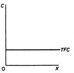
Fixed costs are those which are independent of output. They must be paid even if the firm produces no output. They will not change even if output changes. They remain fixed whether output is large or small. Fixed costs are also called “overhead costs” or “supplementary costs”. They include such payments as rent, interest, insurance, depreciation charges, maintenance costs, property taxes, administrative expense like manager’s salary and so on. In the short period, the total amount of these fixed costs will so on. In the short period, the total amount of these fixed costs will not increase or decrease when the volume of the firms output rises or falls
Fixed Cost = Overhead Cost = supplementary cost
Variable Cost
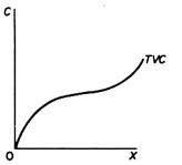
Variable cost are those which are incurred on the employment of variable factors of production. They vary with the level of output. They increase with the rise in output and decrease with the fall in output. By definition variable costs remain zero when output is zero. They include payments for wages, raw materials, fuel, power, transport and the like. Marshall called these variable costs as “Prime Costs” of production.
The relation between total variable cost and output may not be linear, that is, variable cost may not increase by the same amount for every unit increase in output.
Variable Cost = Prime Cost
Total Cost
The total cost (TC) of the firm is a function of output(q). It will increase with the increase with the increase in output, that is, it varies directly with the output. In symbols, it can be written as
TC = f(q)
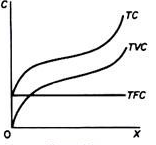
Since the output is produced by fixed and variable factors, the total cost can be dividend into two components: total fixed cost (TFC) and total variable cost (TVC).
TC = TFC + TVC
SHORT RUN COST-OUTPUT
In the earlier chapter we have discussed various concepts of cost. We are now familiar with money cost and its various categories such as fixed cost, variable cost , total cost and marginal cost. These costs behave in different ways as production changes. In this chapter we explain cost-output relationship in the short-run and long-run.
Short-run is a period where a firm produces its output within a given capacity. Its cost is divided between fixed and variable cost. Production is varied by changing variable cost. In the short-run, production is subject to law of variable proportion.
With a hypothetical example we explain behaviour of output and costs as shown in table
A Schedule of Short Run Costs-Output
All Costs in Rupees
Quantity q | Total fixed cost TFC | total variable cost TVC | total cost TC=TFC+TVC | marginal cost MC | average fixed cost AFC=TFC/q | average variable cost AVC=TC/q | average total cost ATC=TC/q ATC(AC)=AVC+AFC |
1 | 2 | 3 | 4 | 5 | 6 | 7 | 8 |
0 | 100 | 0 | 100 |
|
|
|
|
1 | 100 | 25 | 125 | 25 | 100 | 25 | 125 |
2 | 100 | 40 | 140 | 15 | 50 | 20 | 70 |
3 | 100 | 50 | 150 | 10 | 33.3 | 16.7 | 50 |
4 | 100 | 70 | 170 | 20 | 25 | 17.5 | 42.5 |
5 | 100 | 100 | 200 | 30 | 20 | 20 | 40 |
6 | 100 | 145 | 245 | 45 | 16.6 | 24.2 | 40.8 |
7 | 100 | 205 | 305 | 60 | 14.3 | 29.3 | 43.6 |
8 | 100 | 285 | 385 | 80 | 12.5 | 35.6 | 48.1 |
9 | 100 | 385 | 485 | 100 | 11.1 | 42.8 | 53.9 |
10 | 100 | 515 | 615 | 130 | 10 | 51.5 | 61.5 |
In table, output (q) in column 1 ranges from 0 to 10.
Total fixed cost (TFC) in column 2 remains the same (Rs.100) throughout production.
Total Variable Cost (TVC) Change from 0 to 515. When there is n production TVC is zero and as the output increases, TVC also increases.
Total Cost (TC) in column 4 is equal to TFC+TVC, which also increase as the output increases. Given the constant TC, change in TC is due to change in TVC. TVC can be obtained by deducing TFC from TC(TVC=TC-TFC).
Marginal Cost (MC) is the additional cost to produce an additional unit of output which is equal to a change in TVC or a change in TC, as ∆TVC=∆TC.
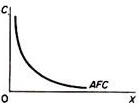
Average Fixed Cost (AFC) is equal to TFC/q. It decline continuously till the last unit of output. This is result of a constant sum (rs.100) which is divided by an increasing denominator.
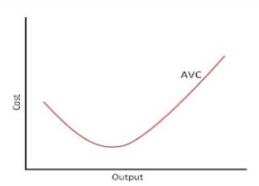
Average Variable Cost (AVC) declines till output 5 (rs.20) and thereafter increases are more units are produced.
Average Total Cost (ATC) is equal to AFC+AVC. It declines till the 5th unit and thereafter increases.
LONG-RUN COST OUTPUT
The long-run is a period of time during which the firm can alter its size and organisation to changing demand conditions. In other words, in the long-run the firm can adjust its scale of operations or size of plant to produce any required output in the most efficient way. Thus, in the long run the fixed factors can be altered. Management can be reorganized to run a firm of a different size. Capital can also be used differently. In short, all factors are variable in the long run and therefore the scale of operations can be altered.
Thus, in the long-run all costs are variable (i.e. the firm faces no fixed costs). The length of time of the long run depends on the industry. In some services industries, such as dry-cleaning, the period of the long-run may be only a few months or weeks. For capital intensive industries, such as electricity-generating plant, the construction of a new plant may take many years and hence long-run may be many years. The length of time of the long-run depends upon the time required for the firm to be able to vary all inputs.
The long-run is often referred to as the planning horizon because the firm can build the plant that minimizes the cost of producing any anticipated level of output. Once the plant has been built, the firm operates I the short-run. Thus, the firm plans for the long-run and operates in the short-run.
Traditional theory
Traditional theory distinguishes between the short run and the long run. In short run some factors are considered fixed ie capital equipment and entrepreneurship are fixed
In long run all the factors are variable
In traditional theory, firm cost are divided into fixed and variable cost
TC = TFC + TVC
Fixed cost are those cost which do not change with the change in the quantity of output. It includes salaries, depreciation, Expenses for building depreciation and repairs, Expenses for land maintenance and depreciation if any

Variable costs are cost which varies as the level of output varies. If output falls the cost falls, if output increase the cosy also increases. It includes cost of raw material, running cost, and cost of direct labour.

Relationship between total, fixed and variable cost
Total cost is obtained by adding total fixed cost (TFC) and total variable cost (TVC).

Average cost
Per unit cost of a goods is called its average cost
Average fixed cost is comprises of two types of cost in the short period
Average fixed cost
The average fixed cost is obtained by dividing TFC by the level of output

Average fixed cost decreases as the output increases.
Average variable cost
The average variable cost is found by dividing the TVC with the corresponding level of output

Marginal cost
Addition made to the total cost by the production of one more unit of a commodity is called marginal cost. Its formula is
Or
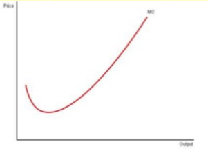
In summary, the traditional theory of costs in the short run shows the cost curves (AVC, ATC and MC) is U-shaped, reflecting the law of variable proportions. In the short run with a fixed plant falling unit cost result in increasing productivity and increasing unit costs result in decreasing productivity.
2. Long run cost of traditional theory
Each firm operates under short run production conditions, but it formulates long run production plans. Study of long run production plan will help in knowing about the production plans of a firm.
No cost is fixed in long run. In this period all cost becomes variable cost. There are three concept of cost in the long run as follows

b. Long run average cost – the long run average cost LRAV shows the minimum or lowest average total cost at which a firm can produce any level of output in the long run. In the traditional theory of the firm the LAC curve is U-shaped and it is often called the ‘envelope curve’

c. Long run marginal cost – LRMC is the minimum increase in total cost associated with an increase in one unit of output when all units are variable. The long run marginal cost is shaped by returns of scale
The LRMC is formed from points of intersection of the SMC curves with vertical lines (to the X-axis) drawn from the points of tangency of the corresponding SAC curves and the LRA cost curve. The LMC must be equal to the SMC for the output at which the corresponding SAC is tangent to the LAC.
The modern theory of cost
According to traditional theory of cost curve, cost curves are U shaped. But according to modern theory the cost curve are L shaped. Modern theory is also based on two time periods i.e. (i) Short Run and (ii) Long Run.
the short run average variable costs curve is saucer – shaped according to modern theory. Over the range of product it has a flat stretch. Flat stretch represents the built in reserve capacity of the plant. The reasons for keeping reserves capacity is to meet seasonal and cyclical fluctuations in demand, change in technology, etc.

ii.short run average cost curve
According to modern theory, AC falls continuously up to a given point as shown in the below figure and then AC is rising upward. It means beyond the reserved capacity AC will rise if output is increased.
iii.short run marginal cost
MC is below to AVC in the beginning. Point P to J marginal cost is horizontal which mean AVC=MC. MC rises above to AVC, after point J as shown below

Long run cost curves
Long run cost curve are L shaped in the modern theory.
The main causes of L – shape of LAC are Technological Progress and Learning by doing

b. Long run marginal cost
The shape of MC is dependent on the relation between LAC and LMC respectively.
As shown in the below fig, when LAC Curve is of inverted J-shaped then LMC is below than LAC Curve. When LAC is constant, LMC also become constant.
