UNIT – 5
Analysis of time series
Introduction
A time series is set of data collected at successive point in a time or over successive period of time. A time series is a collection of observations made sequentially through time. The interval between observations can be any time interval (hours within days, weeks, months, years, etc.).
Some examples of time series are:
analysis.
COMPONENT OF TIME SERIES
Fluctuation in a time series is mainly due to four basic components.
1 Secular trend or trend (T)
2 Seasonal variation (S)
3 Cyclical variation or cyclic fluctuation (C)
4 Irregular or random moments (I)
Secular trend or trend (T)
Upward sloping trend paths in a real- value time series may be indicative of growth phenomenon, a downward sloping path suggest contraction.
3. In a money-value time series an upward sloping path may represent some combination of real growth and inflation; a downward sloping trend path might indicate contraction with deflation.
4. Trend is usually the result of long-term factors such as changes in the population, demographics, technology, or consumer preferences.
Seasonal Variation
5. This is the pattern of variation within time series which repeat itself year to year.
6. Seasonality may be associated with agricultural functions, seasonal weather pattern, custom and convention, or religious or secular holidays.
Cyclic Components:
Irregular Variation
How the component relates to the original series?
A model that expresses the time series variable Y in terms of the components T (trend), C (cycle), S (seasonal) and I (irregular).
Key Takeaways:
Method of least Squares and curve fitting | ||||||||||||||||||||
| Linear tend | |||||||||||||||||||
It is a mathematical method and with it gives a fitted trend line for the set of data in such a manner that the following two conditions are satisfied.
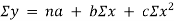
This method gives the line which is the line of best fit. This method is applicable to give results either to fit a straight-line trend or a parabolic trend. The method of least squares as studied in time series analysis is used to find the trend line of best fit to a time series data. Secular Trend Line The secular trend line (Y) is defined by the following equation: Y = a + b X Where, Y = predicted value of the dependent variable a = Y-axis intercept i.e. the height of the line above origin (when X = 0, Y = a) b = slope of the line (the rate of change in Y for a given change in X) When b is positive the slope is upwards, when b is negative, the slope is downwards X = independent variable (in this case it is time) To estimate the constants a and b, the following two equations have to be solved simultaneously: ΣY = na + b ΣX ΣXY = aΣX + bΣX2
To simplify the calculations, if the midpoint of the time series is taken as origin, then the negative values in the first half of the series balance out the positive values in the second half so that ΣX = 0. In this case, the above two normal equations will be as follows: ΣY = na ΣXY = bΣX2
| ||||||||||||||||||||
Example: Below are given the figures of production (in thousand quintals) of a sugar factory: | ||||||||||||||||||||
| ||||||||||||||||||||
(a) Fit a straight-line trend to these figures. (b) Plot these figures on a graph and show the trend line. (c) Estimate the production in 2001.
| ||||||||||||||||||||
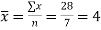
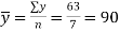
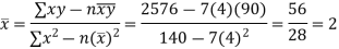
(a) Using normal equations and the sugar production data we can compute constants a and b as shown in Table 7.6: Table : Calculations for Least Squares Equation
| ||||||||||||||||||||
| ||||||||||||||||||||
| ||||||||||||||||||||
| ||||||||||||||||||||
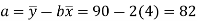
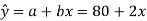
Therefore, linear trend component for the production of sugar is: | ||||||||||||||||||||
| ||||||||||||||||||||
| ||||||||||||||||||||
| ||||||||||||||||||||
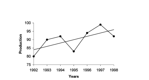
Fig.7.4: Linear Trend for Production of Sugar | ||||||||||||||||||||
| ||||||||||||||||||||
Plotting points on the graph paper, we get an actual graph representing production of sugar over the past 7 years. Join the point a = 82 and b = 2 (corresponds to 1993) on the graph we get a trend line as shown in Fig. 7.4. | ||||||||||||||||||||
| ||||||||||||||||||||
The production of sugar for year 2001 will be
| ||||||||||||||||||||
Parabolic Trend Model
| ||||||||||||||||||||
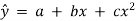
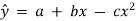
The curvilinear relationship for estimating the value of a dependent variable y from an independent variable x might take the form | ||||||||||||||||||||
| ||||||||||||||||||||
This trend line is called the parabola.
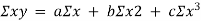
For a non-linear equation
| ||||||||||||||||||||
| ||||||||||||||||||||
| ||||||||||||||||||||
| ||||||||||||||||||||
Example : The prices of a commodity during 1999-2004 are given below. Fit a parabola to these data. Estimate the price of the commodity for the year 2005.
Also plot the actual and trend values on a graph.
| ||||||||||||||||||||
Exponential trend model | ||||||||||||||||||||
Logarithm y = aebx. The equation is
Key Takeaways:
Y = a + b X | ||||||||||||||||||||


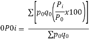
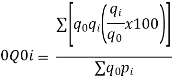
An alternative system of assigning weights lies in using value weights. The value weight | ||||||||||||||||||
| …………….. (6-23) | |||||||||||||||||
then | ||||||||||||||||||
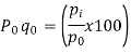
the product of the base period prices and the base period quantities denoted as
| ||||||||||||||||||
the product of the base period prices and the given period quantities denoted as | ||||||||||||||||||
When | ||||||||||||||||||
| …………….. (6-24) | |||||||||||||||||
It may be seen that Similarly, When | ||||||||||||||||||
| ……….. (6-25) | |||||||||||||||||
| ||||||||||||||||||
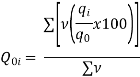
It may be seen that If the index of weighted average of quantity relatives is defined as | ||||||||||||||||||
| …….. (6-26) | |||||||||||||||||
then v can be obtained either as | ||||||||||||||||||
the product of the base period quantities and the base period prices denoted as
| ||||||||||||||||||
the product of the base period quantities and the given period prices denoted as | ||||||||||||||||||
When | ||||||||||||||||||
| …….. (6-27) | |||||||||||||||||
It may be seen that Similarly, When | ||||||||||||||||||
| …….. (6-28) | |||||||||||||||||
It may be seen that | ||||||||||||||||||
| ||||||||||||||||||
Example 6-5 | ||||||||||||||||||
From the data in Example 6.2 find the: | ||||||||||||||||||
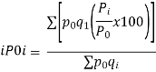
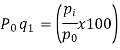
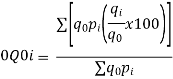
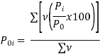
Index of Weighted Average of Price Relatives, using (i) (ii) | ||||||||||||||||||
| ||||||||||||||||||
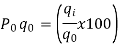
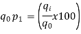
Index of Weighted Average of Quantity Relatives, using (i) (ii)
| ||||||||||||||||||
Calculations for Index of Weighted Average of Price Relatives (Base Year = 1980)
| ||||||||||||||||||
| ||||||||||||||||||
Index of Weighted Average of Price Relatives, using | ||||||||||||||||||
(i) | ||||||||||||||||||
|
|
| ||||||||||||||||
|
|
| ||||||||||||||||
|
|
| ||||||||||||||||
| ||||||||||||||||||
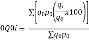
(ii) | ||||||||||||||||||
|
|
| ||||||||||||||||
|
|
| ||||||||||||||||
|
|
| ||||||||||||||||
Calculations for Index of Weighted Average of Quantity Relatives (Base Year = 1980)
| ||||||||||||||||||
| ||||||||||||||||||
Index of Weighted Average of Quantity Relatives, using | ||||||||||||||||||
(i) | ||||||||||||||||||
|
|
| ||||||||||||||||
|
|
| ||||||||||||||||
|
|
| ||||||||||||||||
(ii) | ||||||||||||||||||
|
|
| ||||||||||||||||
|
|
| ||||||||||||||||
|
|
| ||||||||||||||||
| ||||||||||||||||||
Although the indices of weighted average of price/quantity relatives yield the same results as the Laspeyre's or Paasche's price/quantity indices, we do construct these indices also in situations when it is necessary and advantageous to do so. Some such situations are as follows: | ||||||||||||||||||
When a group of commodities is to be represented by a single commodity in the group, the price relative of the latter is weighted by the group as a whole. | ||||||||||||||||||
Where the price/quantity relatives of individual commodities have been computed, these can be more conveniently utilised in constructing the index. | ||||||||||||||||||
Price/quantity relatives serve a useful purpose in splicing two index series having different base periods.
Key Takeaways: | ||||||||||||||||||
| ||||||||||||||||||
| ||||||||||||||||||


Reversal Test
There are two types of test which the different methods of index numbers can be put to check: Time Reversal Test and Factor Reversal Test
A test that may be used under the axiomatic approach which requires that if the prices and quantities in the two periods being compared are interchanged the resulting price index is the reciprocal of the original price index. |
The time reversal test requires that the index for the later period based on the earlier period should be the reciprocal of that for the earlier period based on the later period; one of the desirable features of the “Fisher Ideal” price and volume indexes is that they satisfy this test.
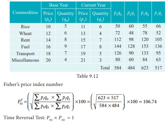
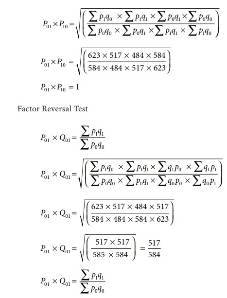
Time Reversal Test
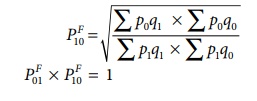
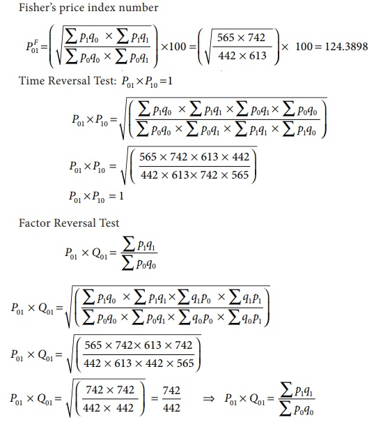
It is an important test for testing the consistency of a good index number. This test maintains time consistency by working both forward and backward with respect to time (here time refers to base year and current year). Symbolically the following relationship should be satisfied, P01 × P10 =1
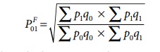
Fisher’s index number formula satisfies the above relationship

when the base year and current year are interchanged, we get
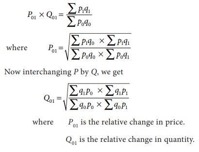
Factor Reversal Test
This is another test for testing the consistency of a good index number. The product of price index number and quantity index number from the base year to the current year should be equal to the true value ratio. That is, the ratio between the total value of current period and total value of the base period is known as true value ratio. Factor Reversal Test is given by,
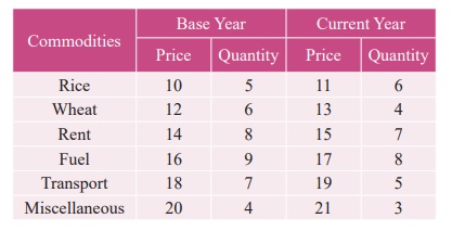
Example 1
Calculate Fisher’s price index number and show that it satisfies both Time Reversal Test and Factor Reversal Test for data given below.
Solution
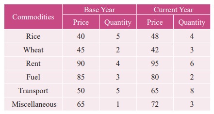
Example 2
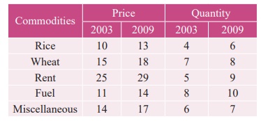
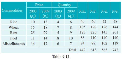
Calculate Fisher’s price index number and show that it satisfies both Time Reversal Test and Factor Reversal Test for data given below.
Solution
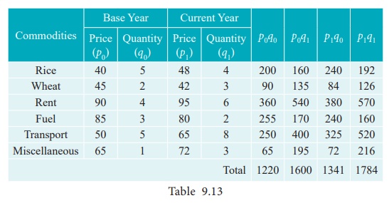
Example 3
Construct Fisher’s price index number and prove that it satisfies both Time Reversal Test and Factor Reversal Test for data following data.
Solution
Key Takeaways:
REFERENCE


