Unit 5
The Sampling Theorem
Sampling theorem states that for a continuous form of a time-variant signal it can be represented in the discrete form of a signal with help of samples and the sampled (discrete) signal can be recovered to original form when the sampling signal frequency Fs having the greater frequency value than or equal to the input signal frequency Fm.
If the sampling frequency (Fs) equals twice the input signal frequency (Fm), then such a condition is called the Nyquist Criteria for sampling. When sampling frequency equals twice the input signal frequency is known as “Nyquist rate”.
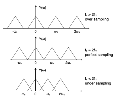
Figure1. Sampling theorem.
Key Takeaways:
- Definition of Sampling theorem
- Its representation .
In time domain, the reconstruction of the continuous signal x(t) from its sampled version xs(t) can be considered as an interpolation process of filling the gaps between neighbouring samples. The interpolation can be considered as convolution of xs(t) with a certain function h(t):
x(t) reconstructed = h(t) * xs(t)
In frequency domain, the interpolation can be considered as a filtering process:
X(w) reconstructed = H(w) Xs(w)
With the general effect of reserving the central portion of the periodic spectrum Xs(w) while suppressing all its replica at higher frequencies.
- Zero-order hold
Ho(t) = { 1 0  t < Ts
0 otherwise
A continuous signal xo(t) can be recovered by
Xo(t) = ho(t) *xs(t)
Which is a series of square pulses with their heights modulated by x(mTs). The interpolation corresponds a low-pass filtering in frequency domain by
Ho(w) = F{ho(t)] = 2/w sin(wTs/2) e -jwTs/2
First-order hold
h1(t) = { 1-|t|/Ts 0 |t|<Ts
0 otherwise
A continuous signal x1(t) can be recovered by
x1(t) = h1(t) * xs(t)
Which is the linear interpolation of the sample train x(mTs) (connecting every two consecutive samples by a straight line). This interpolation corresponds a low-pass filtering in frequency domain by
H1(w) = F [h1(t)] = 4/ w 2 Ts sin 2 (wTs/2)
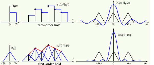
Figure 2. Zero order and first order hold.
Key Takeaways:
- Reconstruction in time and frequency domain
- Zero order and first order hold.
Aliasing can be referred to as “the phenomenon of a high-frequency component in the spectrum of a signal, taking on the identity of a low-frequency component in the spectrum of its sampled version.”
The corrective measures taken to reduce the effect of Aliasing are −
- In the transmitter section of PCM, a low pass anti-aliasing filter is employed, before the sampler, to eliminate the high frequency components, which are unwanted.
- The signal which is sampled after filtering, is sampled at a rate slightly higher than the Nyquist rate.
This choice of having the sampling rate higher than Nyquist rate, also helps in the easier design of the reconstruction filter at the receiver.
Key Takeaways:
- Definition of aliasing
- Its effects and measures
By sampling a continuous-time signal as shown in the figure.
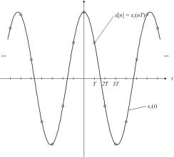
Figure 3. Sampling of continuous signal
Mathematically, the relationship between the discrete-time signal and the continuous-time signal is given by:
x[n] = xc(nT)
The sampling frequency is fs = 1/T or Ωs= 2π/T.
The discrete-time Fourier transform of x[n] is related to the continuous-time Fourier transform of xc(t) as follows:
X(w) = 1/T  (w/T + 2πk/T)
There are two key pieces to this equation.
The first is a scaling relationship between w and Ω : w=Ω T.
This means that the sampling frequency in the continuous-time Fourier transform, Ωs , becomes the frequency 2π in the discrete-time Fourier transform. The discrete-time frequency w=π corresponds to half the sampling frequency, or Ωs/2 .
The second key piece of the equation is that there are an infinite number of copies of Xc(w/T) spaced by 2π .
Suppose Xc(Ω) looks like this:
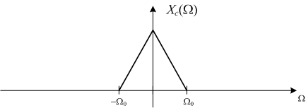
Figure4. Scaling relationship
Note that Xc(Ω) equals zero for all frequencies |Ω|  Ωo. This is what we mean when we say a continuous-time signal is band-limited. The frequency Ωo is called the bandwidth of the signal.
The discrete-time Fourier transform of x[n] = xc[nT] looks like this:
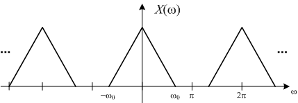
Figure5. Infinite frequencies.
Where wo = ΩoT. X(w) is as shown in figure.
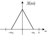
Figure6. Scaled version
For this example, then, X(w) between -π and π looks just like a scaled version of Xc(Ω) .
Key Takeaway:
- Relation of continuous and discrete time systems
- Different applications and mathematical representation
References:
1. A.V. Oppenheim, A.S. Willsky and I.T. Young, "Signals and Systems," Pearson, 2015.
2. R.F. Ziemer, W.H. Tranter and D.R. Fannin, "Signals and Systems - Continuous and Discrete," 4th edition, Prentice Hall, 1998.
3. B.P. Lathi, "Signal Processing and Linear Systems," Oxford University Press, 1998.
4. Douglas K. Lindner, "Introduction to Signals and Systems," McGraw Hill International Edition: 1999.
5. Simon Haykin, Barry van Veen, "Signals and Systems," John Wiley and Sons (Asia) Private Limited, 1998.
6. V. Krishnaveni, A. Rajeswari, “"Signals and Systems," Wiley India Private Limited, 2012.
7. Robert A. Gabel, Richard A. Roberts, "Signals and Linear Systems," John Wiley and Sons, 1995.
8. M. J. Roberts, "Signals and Systems - Analysis using Transform methods and MATLAB," TMH, 2003.
9. J. Nagrath, S. N. Sharan, R. Ranjan, S. Kumar, "Signals and Systems," TMH New Delhi, 2001.
10. A. Anand Kumar, “Signals and Systems,” PHI 3rd edition, 2018.
11. D. Ganesh Rao, K.N. Hari Bhat, K. Anitha Sheela, “Signal, Systems, and Stochastic Processes,” Cengage publication, 2018