Unit-2
Applications of partial differential equation
The second-order PDE in two independent variables of the form
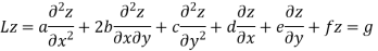
Here a, b, c, d, e, f and g are the functions of the independent variables x and y.
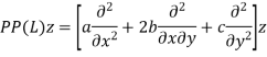
The principal part of the operator L can be given as-
The equation is classified as-
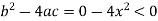
Hyperbolic if- 
Parabolic if- 
Elliptic if- 
Here  is the discriminant of the operator L.
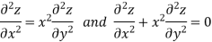
Example: Classify the following PDEs into hyperbolic, parabolic, or elliptic.
Sol. In the first PDE, a = 1, b = 0 and c = 
So that-
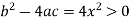
Thus we can say that the given PDE is hyperbolic.
Now in the second PDE,
A = 1, b = 0 and c = 
So that-
Therefore, the second PDE is elliptic.
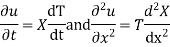
Method of separation of variables
In this method, we assume that the dependent variable is the product of two functions, each of which involves only one of the independent variables. So to ordinary differential equations are formed.
Example 1. Using the method of separation of variables, solve

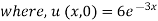
Solution. 
Let, u = X(x). T (t). (2)
Where X is a function of x only and T is a function of t only.
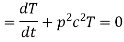
Putting the value of u in (1), we get

(a) 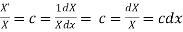
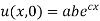
On integration log X = cx + log a = log 


(b)
On integration 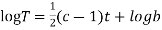
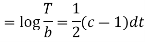
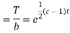

Putting the value of X and T in (2) we have

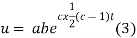
But, 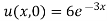
i.e. 
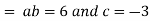
Putting the value of a b and c in (3) we have
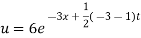

Which is the required solution.
Example 2. Use the method of separation of variables to solve the equation

Given that v = 0 when t→ as well as v =0 at x = 0 and x = 1.
Solution. 
Let us assume that v = XT where X is a function of x only and T that of t only
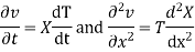
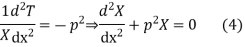
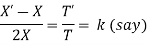
Substituting these values in (1), we get

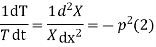
Let each side of (2) equal to a constant 
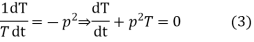
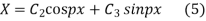
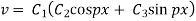
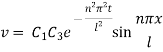
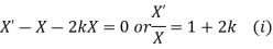
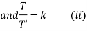
Solving (3) and (4) we have

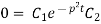
Putting x = 0, v = 0 in (5) we get
On putting the value of  in (5) we get

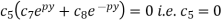
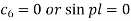
Again putting x = l, v= 0 in (6) we get
Since  cannot be zero.
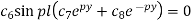
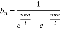
Inputting the value of p in (6) it becomes
Hence, 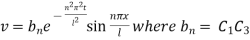
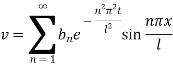
This equation satisfies the given condition for all integral values of n. Hence taking n = 1, 2, 3,… the most general solution is
Example 3. Using the method of separation of variables, solve  Where
Where 
Solution. Assume the given solution 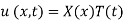
Substituting in the given equation, we have

Solving (i) 
From (ii) 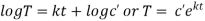
Thus 
Now, 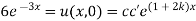

Substituting these values in (iii) we get

Which is the required solution
D'Alembert's solution of the wave equation
The method of d'Alembert provides a solution to the one-dimensional wave equation
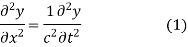
that model's vibrations of a string.
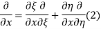
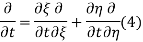
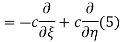
The general solution can be obtained by introducing new variables  and
and  , and applying the chain rule to obtain

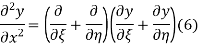
Using (4) and (5) to compute the left and right sides of (3) then give
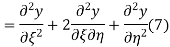
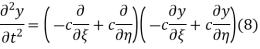
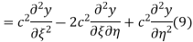
respectively, so plugging in and expanding then gives
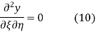
This partial differential equation has the general solution
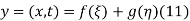

where f and g are arbitrary functions, with f representing a right-traveling wave and g a left-traveling wave.
The initial value problem for a string located at position 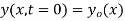 as a function of distance along the string x and vertical speed
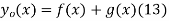
  can be found as follows. From the initial condition and (12),
Taking the derivative with respect to  then gives
and integrating gives
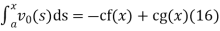
Solving (13) and (16) simultaneously for f and g immediately gives
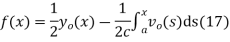
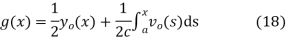
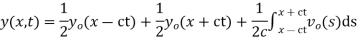
so plugging these into (13) then gives the solution to the wave equation with specified initial conditions as
Example. Find the deflection of a vibrating string of unit length having fixed ends with initial velocity zero and initial deflection f (x)=k (sinx –sin2x)
Solution. By d’Alembert’s method, the solution is
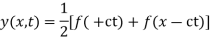

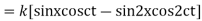

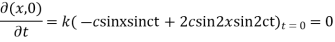
i.e., the given boundary corrections are satisfied.
Wave equation in two dimensions-
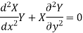
The equation
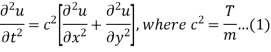
Is the wave equation in two dimensions.
The solution of the wave equation in two dimensions (rectangular membrane)-
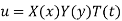
Let us assume that the solution of the above equation (1) is of the form-
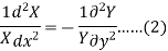
Put these values in the equation and dividing by XYT, we get-
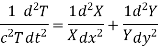
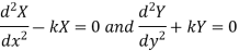
If each member is a constant then this can hold good.
Now choosing the constants suitably, we get-
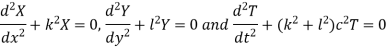
Hence the solution of equation (1) is-

Now let the membrane is rectangular and it is stretched between the lines x = 0, x = a, y = 0, y = b.
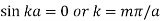
Then the condition u = 0 when x = 0 gives-

Then putting  in (2) and applying the condition u = 0, when x = a,we get-
Now applying the conditions u = , when y = 0 and y = b, we get
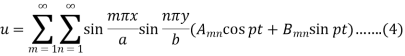
Therefore the solution (2) becomes-

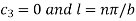
Where 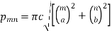
Choosing the constant  so that
We can write the general solution of the equation-1 as-
If the membrane starts from rest from the initial position u = f(x,y)
Which means-
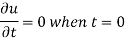
Then equation 3 gives-

Also using the condition u = f(x, y) when t = 0, we get-
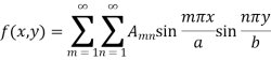
Which is the double Fourier series.
Now multiply both sides by  and integrating from x = 0 to x = a and y = 0 to y = b,
Every term on the right except one, become 0, therefore we get-
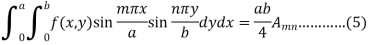
This is called the generalised Euler’s formula.
Example: Find the deflection u(x,y,t) of the square membrane with a = b = 1 and c = 1. If the initial velocity is zero and the initial deflection is f(x, y) = 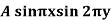 .
.
Sol.
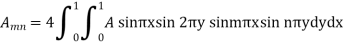
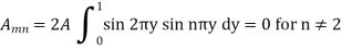
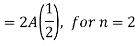
Here taking a = b = 1 and f(x, y) = 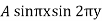 in equation above (5)-
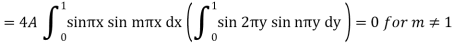
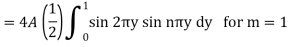
We get-

Also from equation (3) above-
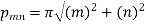
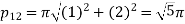
Therefore from equation (4),
The solution will be-

One dimensional heat flow
Let heat flow along a bar of the uniform cross-section in the direction perpendicular to the cross-section. Take one end of the bar as the origin and the direction of the heat flow is along the x-axis.
Let the temperature of the bar at any time t at a point x distance from the origin be u(x,t). Then the equation of one-dimensional heat flow is 
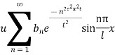
Example 1. A rod of length 1 with insulated sides is initially at a uniform temperature u. Its ends are suddenly cooled to 0° Celsius and are kept at that temperature. Prove that the temperature function u (x, t) is given by
Where  is determined from the equation.
Solution. Let the equation for the conduction of heat be

Let us assume that u = XT, where X is a function of x alone and T that of t alone.
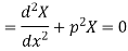
Substituting these values in (1) we get 
i.e. 
Let each side be equal to a constant 

And 
Solving (3) and (4) we have

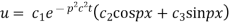
Putting x = 0, u = 0 in (5), we get

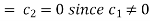
(5) becomes 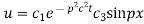
Again putting x = l, u =0 in (6), we get

Hence (6) becomes 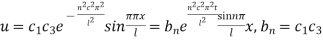
This equation satisfies the given conditions for all integral values n. Hence taking n = 1, 2, 3,…, the most general solution is
By initial conditions 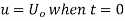

Example 2. Find the solution of

For which u ( 0, t) = u (l.t) =0 =sin  bi method of variable separable.
Solution. 
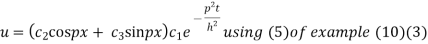
In example 10 the given equation was

On comparing (1) and (2) we get 
Thus the solution of (1) is
On putting x =0
u =0 in (3) we get
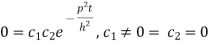
(3) reduced to
On putting x = l and u =0 in (4) we get
Now (4) is reduced to
On putting t = 0, u = 
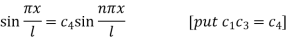
This equation will be satisfied if
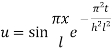
On putting the values of  and n in (5) we have
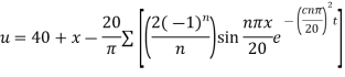
Example 3. The ends A and B of a rod 20 cm long having the temperature at 30 degrees Celsius and 80 degrees Celsius until steady-state prevails. The temperature of the ends is changed to 40 degree Celsius and 60 degree Celsius respectively. Find the temperature distribution in the rod at time t.
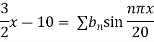
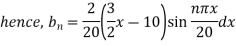
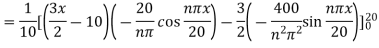
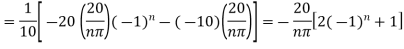
Solution. The initial temperature distribution in the rod is

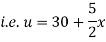
And the final distribution (i.e. steady-state) is
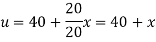
To get u in the intermediate period, reckoning time from the instant when the end temperature was changed we assumed
Where  is the steady-state temperature distribution in the rod (i.e. temperature after a sufficiently long time) and
  is the transient temperature distribution which tends to zero as t increases.
Thus, 
Now  satisfies the one-dimensional heat flow equation

Hence u is of the form

Since 

Hence 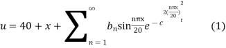
Using the initial condition i.e.
Putting this value of  n (1), we get
Two-dimensional heat flow-
Let us consider the heat flow in a metal plate of uniform thickness, in the direction parallel to the length and breadth of the plate.
Let u(x, y) be the temperature at any point (x, y) of the plate at time t is given as-
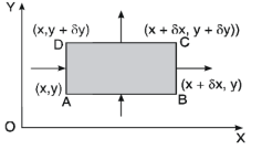
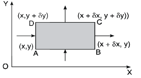
In the steady-state, u doesn’t change with t,

Equation (1) becomes-

Which is known as Laplace’s equation in two dimensions.
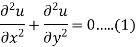
Laplace equation in two dimensions
The equation-

Is known as Laplace’s equation in two dimensions.
The solution of Laplace’s equation-
Let

Put the value in (1), we get-
Separating the variables-
Since x and y are the independent variables, equation (2) can hold good only if each side of (2) is equal to a constant (k),
Then (2) leads the ordinary differential equation-
On solving these equations, we get-


2. When k is negative and it equals to  , say
, say

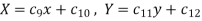
3. When k is zero-
Example: Solve Laplace’s equation  subject to the conditions u(0, y) = u(l, y) = u(x, 0) = 0 and u(x, a) = sin n
Sol.
The three possible solutions of Laplace’s equation-

are-


We need to solve equation (1) satisfying the following boundary conditions-
u(0, y) ........... (5)
u(l, y) = 0........(6)
u(x, 0) = 0 ..........(7)
and u(x, a) = sin n ...... (8)
using (5), (6) and (2), we get-

Solving these equations, we get-

Which leads to a trivial solution.
Similarly, we get a trivial solution by using (5), (6), and (4).
Hence the solution for the present problem is the solution (3).
Now using (5) in (3), we get-
Therefore, equation (3) becomes-

Using (6), we get-
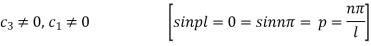
Therefore either-
If we take  then we get a trivial solution.
Thus sin pl = 0 whence 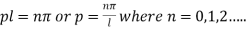
Equation (9) becomes-
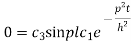
Using (6), we have 0 = 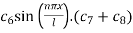
i.e.

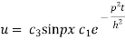
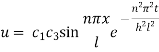
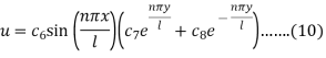
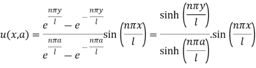
Thus the solution suitable for this problem is-
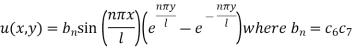
Now using the condition (8)-
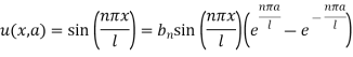
We get-
Hence the required solution is-
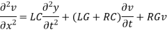
And
Are called telephone equations.

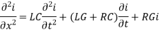
And

Which are called the telegraph equations.
2. If L = G = 0 then,


Are called radio equations.
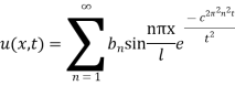
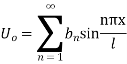
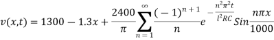
Example: A transmission line 1000 km long is initially under steady-state conditions with potential 1300 volts at the sending end (x = 0) and 1200 volts at the receiving end (x =1000). The terminal end of the line is suddenly grounded but the potential at the source is kept at 1300 volts.
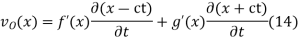
Assuming the inductance and leakage to be negligible, find the potential v(x, t ).
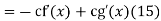
Sol. We know that the equation of the telegraph line is-
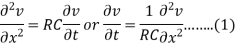


So that-

Where l = 1000 km
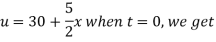
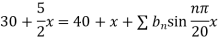
Putting t = 0, we get from (2) and (3)
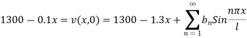
I.e.
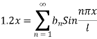
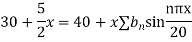
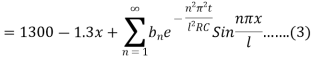
Where-
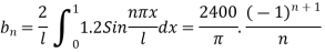
Hence
References
1. Erwin Kreyszig, Advanced Engineering Mathematics, 9thEdition, John Wiley & Sons, 2006.
2. N.P. Bali and Manish Goyal, A textbook of Engineering Mathematics, Laxmi Publications.
3. B.S. Grewal, Higher engineering mathematics, Khanna publishers


