Module-1
Laplace Transform
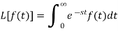
Let f(t) be any function of t defined for all positive values of t. Then the Laplace transform of the function f(t) is defined as-
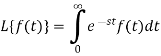
Provided that the integral exists, here ‘s’ is the parameter that could be real or complex.
The inverse of the Laplace transform can be defined as below-

Here 
f(t) is called the inverse Laplace transform of 
L is called the Laplace transformation operator.
Conditions for the existence of Laplace transform-
The Laplace transform of f(t) exists for s>a, if
1. f(t) is a continuous function.
2.  is finite.
Important formulae-
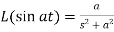
1. 
2. 
3. 
4. 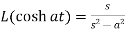
5. 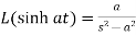
6. 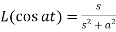
7. 
Example-1: Find the Laplace transform of the following functions-
1.  2.
2. 
Sol. 1.
Here 
So that we can write it as-
Now-
2. Since 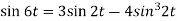
Or 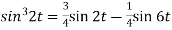
Now-
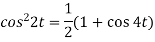
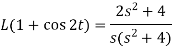
Example-2: Find the Laplace transform of (1 + cos 2t)
Sol. 

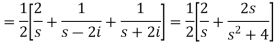
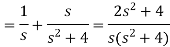
So that-
Properties and theorems of LT
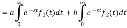
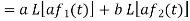
1. Linearity property-
Let a and b be any two constants and  ,
,  any two functions of t, then-

Proof:
Hence proved.
2. First shifting property (Theorem)- If 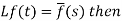
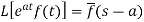
Proof: By definition-
Let (s – a) = r
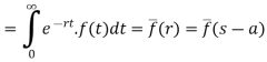
Hence proved.
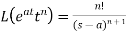
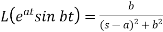
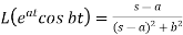
We can find the following results with the help of the above theorem-
1. 
2. 
4. 
5. 
6. 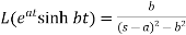
7. 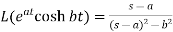
Here s>a in each case.
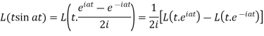
Example-1: Find the Laplace transform of t sin at.
Sol. Here-
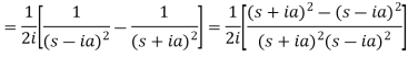
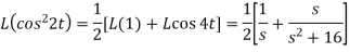
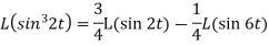
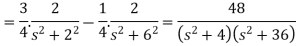
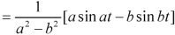
Example-2: Find the Laplace transform of 
Sol. Here-
So that-
As we know that- 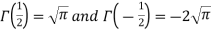
So that-
Hence-
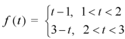
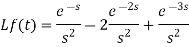
Example-3: Find the Laplace transform of the following function-
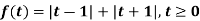
Sol. The given function f(t) can be written as-
So, by definition,
Existence theorem-
The Laplace transform of f(t) exists for s>a if –
- F(t) is continuous
 is finite.
The above conditions are not necessary but sufficient.
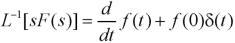
Laplace transform of the derivative of f(t)-
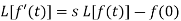
Here 
Proof: by the definition of Laplace transform-

On integrating by parts, we get-
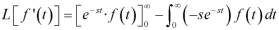
Since 
Then-
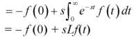
So that-

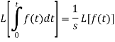
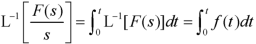
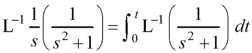
Laplace transform of integral of f(t) -
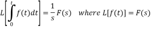
Proof: Suppose
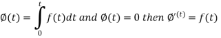
We know that-

So that-
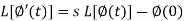
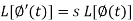
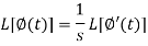
Putting the values of  and
and  , we get-
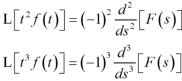
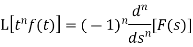
Laplace transform of the function  multiplied by t
If  , then-

Proof: 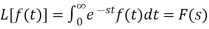
Differentiate w.r.t. x, we get-

Similarly-
And
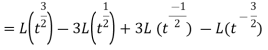
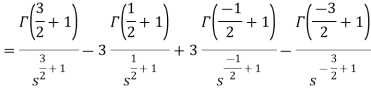
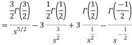
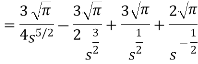
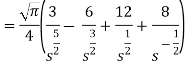
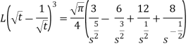
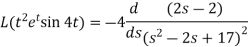
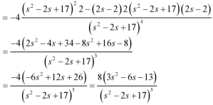
Example-4: Find the Laplace transform of  .
.
Sol. Here-
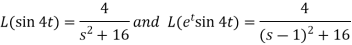
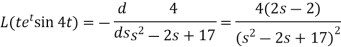
Now-
We can solve the initial value problems directly without first finding a general solution by using the Laplace transform method for solving initial value problems.
Example: solve the initial value problem-
Sol.
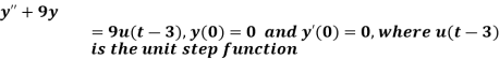
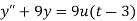
Take the Laplace transform of the given differential equation, we get-

Using the initial conditions, we get-

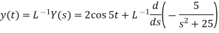
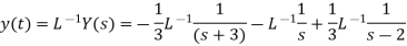
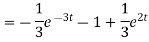
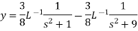
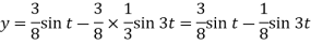
On taking Laplace inverse of Y(s), we get-

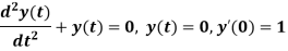
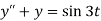
Example: using Laplace transform find the solution of the following initial value problem-
y’’ + 25y = 10 cos 5t, y(0) = 2, y’(0) = 0
Sol.
Here we have-
y’’ + 25y = 10 cos 5t, y(0) = 2, y’(0) = 0
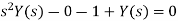
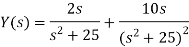
On taking Laplace transform of the given differential equation and using initial conditions, we get-
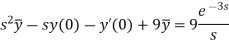
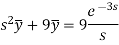
Example: using Laplace transform find the solution of the following initial value problem-
y’ + y = 
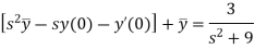
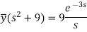
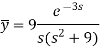
Sol. On taking the Laplace transform and using the initial conditions, we get-

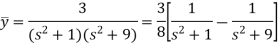
Thus
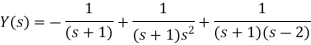
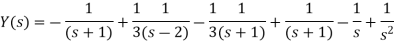
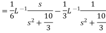
On breaking into partial fractions, we get-
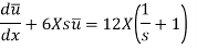
Example: Solve the following initial boundary value problem-

Sol.
Taking Laplace to transform with respect to ‘t’ and using-
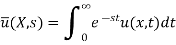
We get-
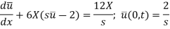
Or
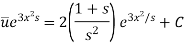
It is a linear ordinary differential equation and its solution is given by-
When x = 0, 
Hence C = 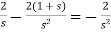
So that-
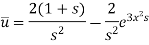
Now taking Laplace inverse of  , we get-

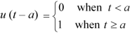
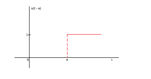
Unit step function
The unit step function u(t – a) is defined as-
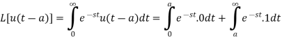
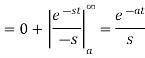
Laplace transform of unit functions-
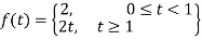
Example-1: Express the function given below in terms of a unit step function and find it's Laplace transform as well-
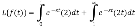
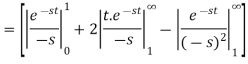
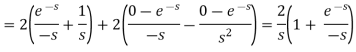
Sol. Here we are given-


So that-
Example-2: Find the Laplace transform of the following function by using unit step function-

Sol. 

Since 

Dirac-delta function-
The impulse function is also known as the Dirac-delta function.
Impulse- When a large force acts for a short time, then the product of the force and the time is called impulse.
The unit impulse function is the limiting function.
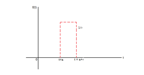
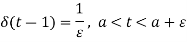
= 0, otherwise
The unit impulse function can be defined as-
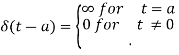
And
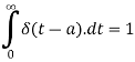
Laplace transform of unit impulse function-
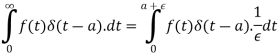
We know that-
Mean value theorem- 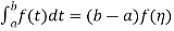
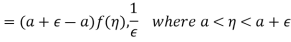

As  , then we get-
When  then we have
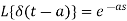
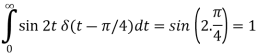
Example-1: Evaluate-
1. 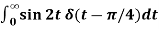

Sol.1. As we know that- 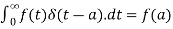
So that-
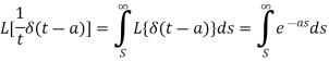
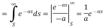
2. As we know that-

Example-2: 
Sol. 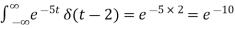
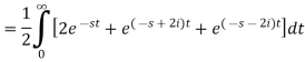
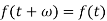
Suppose the function f(t) be periodic with period  , then-

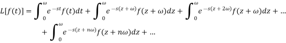
Similarly-

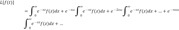
Now-

Put t = z + in the second integral of the above equation and t = z + 2
 in the third integral and so on.
We get-
F(t) is periodic with period  we can write-
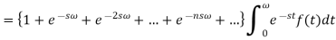
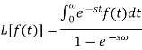
Here  is a geometric progression with a common ratio
  , and we know that the sum of infinite terms in G.P. Is given by
Then-
Inverse Laplace transforms-
The inverse of the Laplace transform can be defined as below-
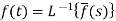
Here 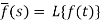
f(t) is called the inverse Laplace transform of 
L is called the Laplace transformation operator.
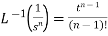
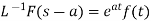
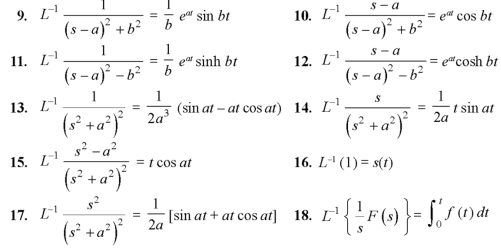
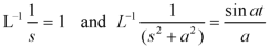
Important formulae-
1.  2.
2. 
3. 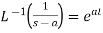 4.
4. 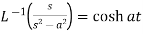
5. 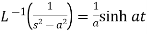 6.
6. 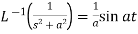
7. 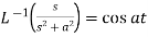 8.
8. 
Example: Find the inverse Laplace transform of the following functions-
1. 
2. 
Sol.
1.
2.
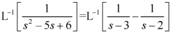
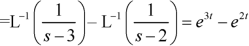
Example: Find the inverse Laplace transform of-

Sol.

Multiplication by ‘s’ -
Example: Find the inverse Laplace transform of-

Sol.

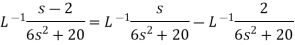
Division by s-
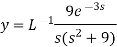
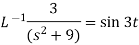
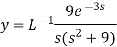
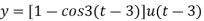
Example: Find the inverse Laplace transform of-

Sol.
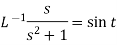
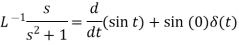
Inverse Laplace transform of derivative-
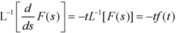
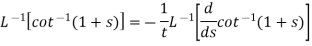
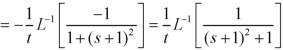
Example: Find 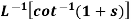
Sol.

Inverse Laplace transform by using partial fraction
We can find the inverse Laplace transform by using the partial fractions method described below-
Example: Find the Laplace inverse of-
Sol.
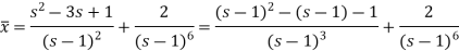
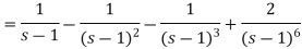
We will convert the function into partial fractions-
Example: Find the inverse transform of-

Sol.
First, we will convert it into partial fractions-
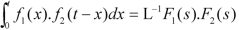
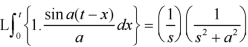
Inverse Laplace transform by convolution theorem-
According to the convolution theorem-
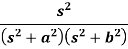
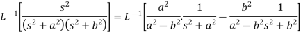
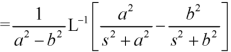
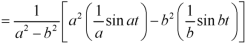
Example: Find

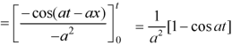
Sol.
Therefore by the convolution theorem-

Step by step procedure to solve a linear differential equation by using Laplace transform-
1. Take the Laplace transform of both sides of the given differential equation.
2. Transpose the terms with a negative sign to the right.
3. Divide by the coefficient of  , getting
  as a known function of s.
4. Resolve the function of s into partial fractions and take the inverse transform of both sides.
We will get y as a function of t. Which is the required solution.
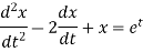
Example-1: Use Laplace transform method to solve the following equation-

Sol. Here we have-
Take Laplace transform of both sides, we get-

It becomes-
(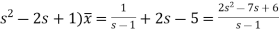
So that-
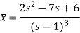
Now breaking it into partial fractions-
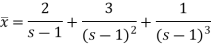
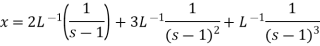
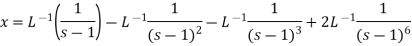
We get the following results on inversion-
Example-2: Use Laplace transform method to solve the following equation-

Sol.
Here, taking the Laplace transform of both sides, we get

It becomes-
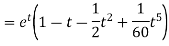
On inversion, we get-
Example-3: Use Laplace transform method to solve the following equation-

Sol. Here we have-
Taking Laplace transform of both sides, we get-
We get on putting given values-
On inversion, we get-
Example-4: Find the solution of the initial value problem by using Laplace transform-
Sol. Here we have-
Taking Laplace transform, we get-
Putting the given values, we get-
On inversion, we get-
 4
4
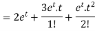
Now-
The solution of simultaneous differential equations by using Laplace transform-
Example: solve the following differential equation by using Laplace transform-
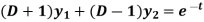

Here D = d/dt and 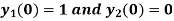
Sol.
Here we have-


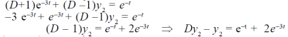
Now multiply (1) by D+1 and (2) by D – 1 we get-


Now subtract (4) from (3), we get-


By taking Laplace to transform we get-
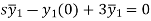


Put the value of  in (1) we get-
By taking Laplace to transform we get-
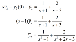
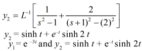
Which is the required answer.
Reference Books
1. B.S. Grewal: Higher Engineering Mathematics; Khanna Publishers, New Delhi.
2. B.V. Ramana: Higher Engineering Mathematics; Tata McGraw- Hill Publishing Company Limited, New Delhi.
3. Peter V.O’ Neil. Advanced Engineering Mathematics, Thomas ( Cengage) Learning.
4. Kenneth H. Rosem: Discrete Mathematics its Application, with Combinatorics and Graph Theory; Tata McGraw- Hill Publishing Company Limited, New Delhi
5. K.D. Joshi: Foundation of Discrete Mathematics; New Age International (P) Limited,
Publisher, New Delhi.


