Module-2

Integral Transform

2.1 Fourier integral, Fourier Transform , Complex Fourier transform

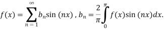
The Fourier integral of f(x) is-

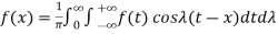………. (1)

Which can be written as-

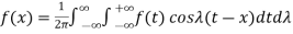  …………… (2)

Because is an even function of . Also since is an odd function of then we have-

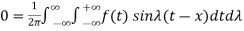  ……… (3)

Multiply (3) by ‘i’ and add to (2)-

We get-

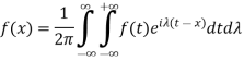
Which is the complex form of the Fourier integral.

Example 1:

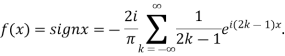
Using the complex form, find the Fourier series of the function

f(x) = sinx =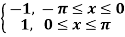

Solution:

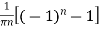
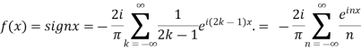
We calculate the coefficients

  =

=

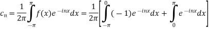
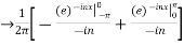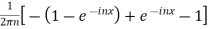
Hence the Fourier series of the function in complex form is

We can transform the series and write it in the real form by renaming it as

n=2k-1,n=

=

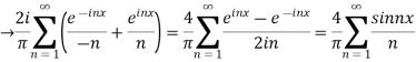
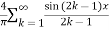
Example 2:

Using complex form find the Fourier series of the function f(x) = x2, defined on the interval [-1,1]

Solution:

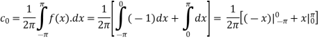
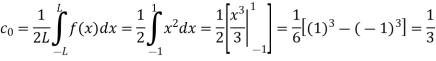
Here the half-period is L=1. Therefore, the coefficient c0 is,

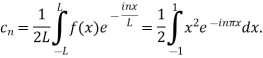
For n

Integrating by parts twice, we obtain

=

=

= .

= .

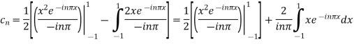
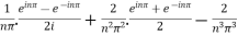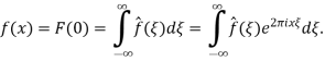
Fourier integral theorem

If   f, then

Proof. We first claim that

Let By the multiplication formula we get

Since is a good kernel, n the first integral goes to f(0) as tends to 0. Since the

The second integral converges to as our claim is proved.

In general , let F(y)=f(y+x) so that

Example:1

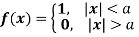
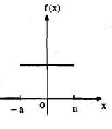
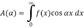
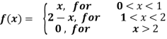
Find the Fourier integral representation of the function

Solution:

The graph of the function is shown in the below figure satisfies the hypothesis of

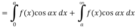
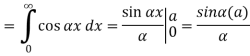
Theorem -1. Hence from Eqn,(5) and (6), we have

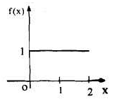
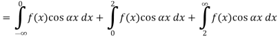
Substituting these coefficients in Eqn. (4) we obtain

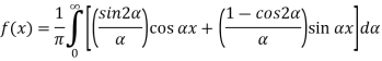
This is the Fourier integral representation of the given function.

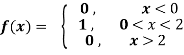
Example:2

Find the Fourier integral representation of the function

Solution:

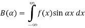
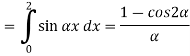
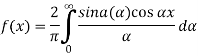
The graph of the given function is shown in the below figure. Clearly, the given function f(x) is an even function. We represent f(x) by the Fourier cosine integral. We obtain

And thus,

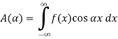
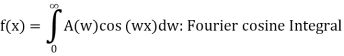
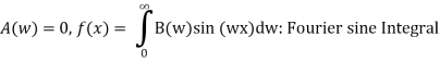
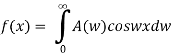
Fourier Sine & Cosine integrals-

The following notations are used to find the Fourier sine and cosine integrals.

If the function f(x) is even      

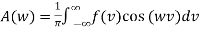
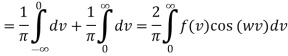
B(w)= 0

If the function f(x) is odd

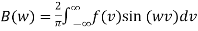
Example:1

Find the Fourier cosine integral of , where x>0, k>0 hence show that

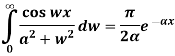
Solution:

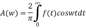
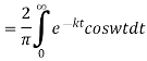
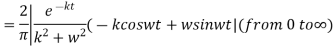
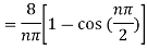
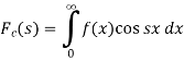
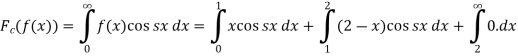
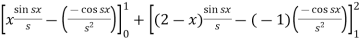
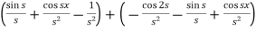
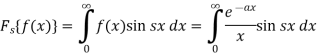
The Fourier cosine integral of f(x) is given by:

Example:2

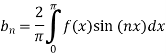
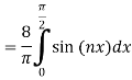
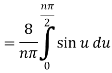
Find the half –range sine series of the function

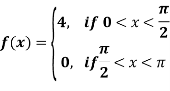
Solution: xx

Where

Fourier transform

In mathematics, a Fourier transform (FT) is a mathematical transform that decomposes a function (often a function of time, or a signal) into its constituent frequencies, such as the expression of a musical chord in terms of the volumes and frequencies of its constituent notes. The term Fourier transform refers to both the frequency domain representation and the mathematical operation that associates the frequency domain representation to a function of time.

The Fourier transform of a function of time is a complex-valued function of frequency, whose magnitude (absolute value) represents the amount of that frequency present in the original function, and whose argument is the phase offset of the basic sinusoid in that frequency. The Fourier transform is not limited to functions of time, but the domain of the original function is commonly referred to as the time domain. There is also an inverse Fourier transform that mathematically synthesizes the original function from its frequency domain representation, as proven by the Fourier inversion theorem

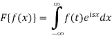
The function-

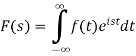
Is called the Fourier transform of the function f(x).

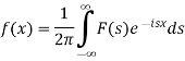
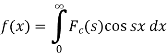
The function f(x) given below is called inverse Fourier transform of F(s)-

Properties of Fourier transform-

Property-1: Linear property- If F(s) and G(s) are two Fourier transforms of f(x) and g(x) respectively, then-

Where a and b are the constants.

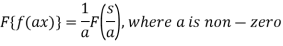
Property-2: Change of scale- If F(s) is a Fourier transform of f(x), then

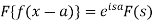
Property-3: Shifting property- If F(s) is a Fourier transform of f(x), then

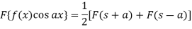
Property-4: Modulation- If F(s) is a Fourier transform of f(x), then

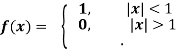
Example: Find the Fourier transform of-

Hence evaluate

Sol. As we know that the Fourier transform of f(x) will be-

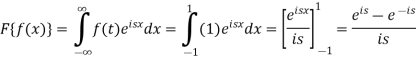
So that-

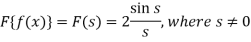
For s = 0, we get- F(s) = 2

Hence by the inverse formula, we get-

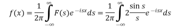
Putting x = 0, we get

So-

Example: Find the Fourier transform of

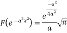
Sol. As we know that the Fourier transform of f(x) will be-

So that-

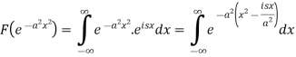
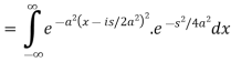
Now put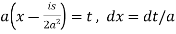

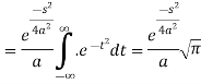
So that-

2.2. Inverse Transforms, Convolution Theorems

The f(x) given below is called the inverse Fourier transform of F(s)-

1. Inverse Fourier sine transform of F(s)-

2.     Inverse Fourier cosine transform of F(s)-

Convolution theorem-

The Fourier transform of the convolution of f (x) and g (x) is the product of their Fourier Transforms.

Which means-

Proof:

We have-

Take Fourier to transform on both sides of the above equation, we get-

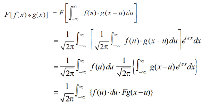
By shifting property-

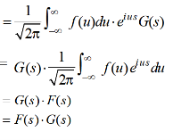
By inversion, we get-

2.3 Fourier sine and cosine transform

Then-

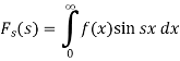
The function is known as the Fourier sine transform of f(x) in 0<x<∞

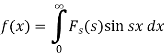
And the function f(x) s called the inverse Fourier sine transform of .

And-

Then

The function is known as the Fourier cosine transform of f(x) in 0<x<∞

And the function f(x) s called the inverse Fourier cosine transform of .

Finite Fourier sine and cosine transforms-

The finite Fourier sine transform of f(x), in 0<x<c, is given by-

Where n is an integer.

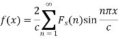
And the function f(x) is called the inverse finite Fourier sine transform of which is defined by-

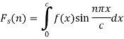
The finite Fourier cosine transform of f(x), in 0<x<c, is given by-

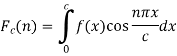
Where n is an integer.

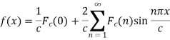
And the function f(x) is called the inverse finite Fourier cosine transform of which is defined by-

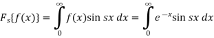
Example-1: Find the Fourier sine transform of

Sol. Here x being positive in the interval (0, ∞)

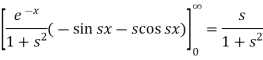
Fourier sine transform of will be-

Example-2: Find the Fourier cosine transform of-

Sol. We know that the Fourier cosine transform of f(x)-

=

= 

=

Example-3: Find the Fourier sine transform of

Sol. Let                    

Then the Fourier sine transform will be-

Now suppose,

Differentiate both sides with respect to x, we get-

……. (1)

On integrating (1), we get-

2.4 Applications of Fourier transform to simple one-dimensional heat transfer equations, Wave equations, and Laplace equations

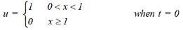
Example: Solve the equation-

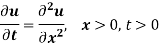
Subject to the conditions-

1. u = 0 when x = 0, t>0
2. 
3. U(x,t) is bounded.

Sol.

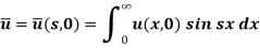
Here we apply Fourier sine transform-

We get-

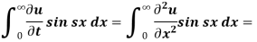
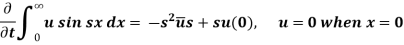
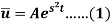
...... (2)

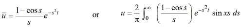
Put the value of in equation (1), we get

So that-

Wave equation-

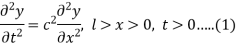
The wave equations are given as-

The solution of the wave equation by Laplace transform-

Example: A uniform rod whose length is ‘l’ at rest in its equilibrium position with the end x = 0 fixed. At t = 0, a constant force per unit, the area is applied at the free end.

Find the motion of the rod for t>0.

Sol.

Suppose the displacement in the rod is y(x,t).

The equation of motion is given by-

Subject to the conditions-

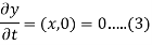
y(x,0) = 0 ..... (2)

y(0,t) = 0 ...... (4)

Here E is Young’s modulus.

Now applying Laplace transform on (1), we get-

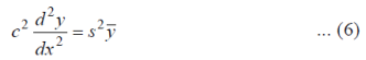
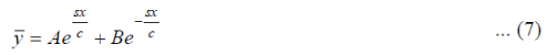
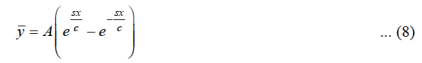
We know that equation (6) is an ordinary differential equation and its solution is-

Put y = 0 and x = 0 from (2) in (7),we get-

0  = A + B

B = -A

Then (7) becomes-

Laplace transform of (3) is-

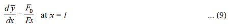
Differentiating equation (8) w.r. t x-

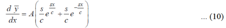
Put the value of from (9) and (10)-

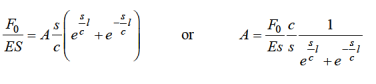
Put the value of A in (8), we get-

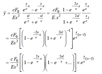
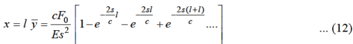
Putting x = l in (11),

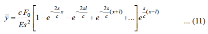
Now applying inversion transform on (12), we get-

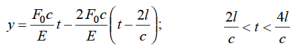
Putting

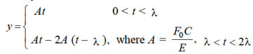
Which is the required answer.

2.5 Z-Transform and its application to solve differential equations.

In mathematics and signal processing, the Z-transform converts a discrete-time signal, which is a sequence of real or complex numbers, into a complex frequency-domain representation. It can be considered as a discrete-time equivalent of the Laplace transform. This similarity is explored in the theory of time-scale calculus.

Analysis of continuous-time LTI systems can be done using z-transforms. It is a powerful mathematical tool to convert differential equations into algebraic equations.

The bilateral (two-sided) z-transform of a discrete-time signal x(n) is given as

Z.T[x(n)] = X(Z) =

The unilateral (one sided) z-transform of a discrete time signal x(n) is given as

Z.T[x(n) = X(Z) =

Z-transform may exist for some signals for which Discrete-Time Fourier Transform (DTFT) does not exist.

Definition

The Z-transform can be defined as either a one-sided or two-sided transform.

Bilateral Z-transform

The bilateral or two-sided Z-transform of a discrete-time signal {\displaystyle x[n]}x(n) is the formal power series {\displaystyle X(z)}X(z)  defined as

X (z) = Z =

Where {\displaystyle n}n is an integer and z{\displaystyle z} is, in general, a complex number:

{\displaystyle z=Ae^{j\phi }=A\cdot (\cos {\phi }+j\sin {\phi })}

Where {\displaystyle A}A is the magnitude of z,j{\displaystyle z} {\displaystyle j} is the imaginary unit and {\displaystyle \phi } is the complex argument (also referred to as angle or phase) in radians.

Unilateral Z-transform

Alternatively, in cases where {\displaystyle x[n]}x[n] is defined only for {\displaystyle n\geq 0} the single-sided or unilateral Z-transform is defined as

X (z) = Z =

In signal processing, this definition can be used to evaluate the Z-transform of the unit impulse response of a discrete-time causal system.

An important example of the unilateral Z-transform is the probability-generating function, where the component {\displaystyle x[n]}x[n] is the probability that a discrete random variable takes the value {\displaystyle n}n, and the function X(z){\displaystyle X(z)} is usually written as {\displaystyle X(s)}X(s) in terms of{\displaystyle s=z^{-1}} s = x-1. The properties of Z-transforms (below) have useful interpretations in the context of probability theory.

Standard properties

Z-transform properties:

Z-Transform has the following properties:

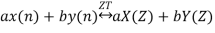
1. Linearity Property

If x(n)X(Z)

And

y(n)Y(Z)

Then linearity property states that

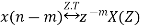
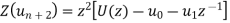
2. Time Shifting Property

Then the time-shifting property states that

Multiplication by Exponential Sequence Property

If x(n)

Then multiplication by an exponential sequence property is

3. Time Reversal Property

If x(n)

Then time reversal property states that

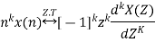
Differentiation in Z-Domain OR Multiplication by n Property

If 

Then multiplication by n or differentiation in z-domain property states that,

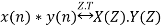
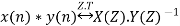
4. Convolution Property

If
 

And

Then convolution property states that

5. Correlation Property

If 

And

Then co-relation property states that

Region of Convergence (ROC) of Z-Transform

The range of variation of z for which z-transform converges is called the region of convergence of z-transform.

Properties of ROC of Z-Transforms

• ROC of z-transform is indicated with a circle in z-plane.
• ROC does not contain any poles.
• If x(n) is a finite duration causal sequence or right-sided sequence, then the ROC is entire z-plane except at z = 0.
• If x(n) is a finite duration anti-causal sequence or left-sided sequence, then the ROC is the entire z-plane except at z = ∞.
• If x(n) is an infinite duration causal sequence, ROC is the exterior of the circle with radius a. i.e. |z| > a.
• If x(n) is an infinite duration anti-causal sequence, ROC is the interior of the circle with radius a. i.e. |z| < a.
• If x(n) is a finite duration two sided sequence, then the ROC is entire z-plane except at z = 0 & z = ∞.

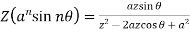
Some standard formulae-

1.

2.

3.

4.

5.

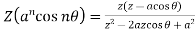
6.

Example-1:Find Z-transform of the following functions-

(i)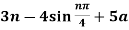

(ii)

Sol. (i) 

(ii)

Example-2: Find Z-transform of the following functions-

(i)

(ii)

Sol. (i) As we know that-

So that-

(ii) we know that-

So that-

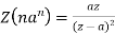
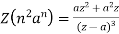
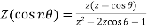
ZT of standard sequences and their inverses

Sequence	z-transformation
	1

Example 1:

Find the z-transformation of the following left-sided sequence

Solution:

= 

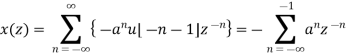
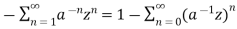
= 1-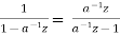

=

If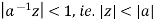 

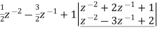
Example 2:

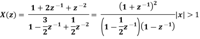
Solution:

Long division method to obtain

2

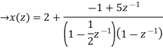
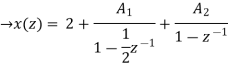
Now x(z) can be written as,

X(z) = 2-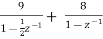

The solution of difference equations

Working procedure to solve the linear difference equation by ZT-

1. Take the ZT of both sides of the differential equations.

2. Transpose all terms without U(z) to the right

3. Divide by the coefficients of U(z)

4. Express this function in terms of the Z-transform of the known function and take the inverse ZT of both sides.

This will give as a function of n, is the required solution.

Example 1:

Solve the differential equation 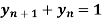 by the z-transformation method.

Solution:

Given,

Let y(z) be the z-transform of

Taking z-transforms of both sides of eq (1) we get,

Ie.

Using the given condition, it reduces to

(z+1) y(z) =

i.e.

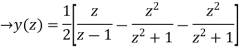
Y(z) =

Or Y(Z) =

On taking inverse Z-transforms, we obtain

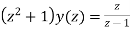
Example 2:

Solve 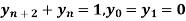using z-transforms

Solution:

Consider,

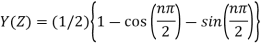
Taking z-transforms on both sides, we get

=

or

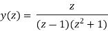
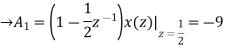
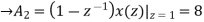
Now,

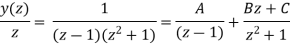
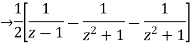
Using inverse z-transform we obtain,

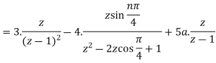
Example-3:

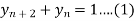
Solve the following by using Z-transform

Sol. If then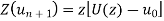

And

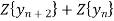
Now taking the Z-transform of both sides, we get

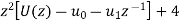z[

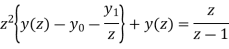
It becomes-

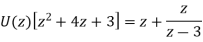
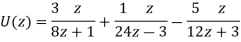
So,

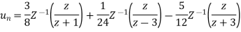
Now-

On inversion, we get-

Reference Books

1. B.S. Grewal: Higher Engineering Mathematics; Khanna Publishers, New Delhi.

2. B.V. Ramana: Higher Engineering Mathematics; Tata McGraw- Hill Publishing Company Limited, New Delhi.

3. Peter V.O’ Neil. Advanced Engineering Mathematics, Thomas ( Cengage) Learning.

4. Kenneth H. Rosem: Discrete Mathematics its Application, with Combinatorics and Graph Theory; Tata McGraw- Hill Publishing Company Limited, New Delhi

5. K.D. Joshi: Foundation of Discrete Mathematics; New Age International (P) Limited,

Publisher, New Delhi.