Unit - 4

Machine Learning

4.1 Supervised and unsupervised learning

Machine Learning (ML) is an automated learning with little or no human intervention. It involves programming computers so that they learn from the available inputs. The main purpose of machine learning is to explore and construct algorithms that can learn from the previous data and make predictions on new input data.

The input to a learning algorithm is training data, representing experience, and the output is any expertise, which usually takes the form of another algorithm that can perform a task. The input data to a machine learning system can be numerical, textual, audio, visual, or multimedia. The corresponding output data of the system can be a floating-point number, for instance, the velocity of a rocket, an integer representing a category or a class, for example, a pigeon or a sunflower from image recognition.

In this chapter, we will learn about the training data our programs will access and how learning process is automated and how the success and performance of such machine learning algorithms is evaluated.

Concepts of Learning

Learning is the process of converting experience into expertise or knowledge.

Learning can be broadly classified into three categories, as mentioned below, based on the nature of the learning data and interaction between the learner and the environment.

• Supervised Learning
• Unsupervised Learning
• Semi-supervised Learning

Similarly, there are four categories of machine learning algorithms as shown below −

• Supervised learning algorithm
• Unsupervised learning algorithm
• Semi-supervised learning algorithm
• Reinforcement learning algorithm

However, the most commonly used ones are supervised and unsupervised learning.

Supervised Learning

Supervised learning is commonly used in real world applications, such as face and speech recognition, products or movie recommendations, and sales forecasting. Supervised learning can be further classified into two types - Regression and Classification.

Regression trains on and predicts a continuous-valued response, for example predicting real estate prices.

Classification attempts to find the appropriate class label, such as analyzing positive/negative sentiment, male and female persons, benign and malignant tumors, secure and unsecure loans etc.

In supervised learning, learning data comes with description, labels, targets or desired outputs and the objective is to find a general rule that maps inputs to outputs. This kind of learning data is called labeled data. The learned rule is then used to label new data with unknown outputs.

Supervised learning involves building a machine learning model that is based on labeled samples. For example, if we build a system to estimate the price of a plot of land or a house based on various features, such as size, location, and so on, we first need to create a database and label it. We need to teach the algorithm what features correspond to what prices. Based on this data, the algorithm will learn how to calculate the price of real estate using the values of the input features.

Supervised learning deals with learning a function from available training data. Here, a learning algorithm analyzes the training data and produces a derived function that can be used for mapping new examples. There are many supervised learning algorithms such as Logistic Regression, Neural networks, Support Vector Machines (SVMs), and Naive Bayes classifiers.

Common examples of supervised learning include classifying e-mails into spam and not-spam categories, labeling webpages based on their content, and voice recognition.

Unsupervised Learning

Unsupervised learning is used to detect anomalies, outliers, such as fraud or defective equipment, or to group customers with similar behaviors for a sales campaign. It is the opposite of supervised learning. There is no labeled data here.

When learning data contains only some indications without any description or labels, it is up to the coder or to the algorithm to find the structure of the underlying data, to discover hidden patterns, or to determine how to describe the data. This kind of learning data is called unlabelled data.

Suppose that we have a number of data points, and we want to classify them into several groups. We may not exactly know what the criteria of classification would be. So, an unsupervised learning algorithm tries to classify the given dataset into a certain number of groups in an optimum way.

Unsupervised learning algorithms are extremely powerful tools for analyzing data and for identifying patterns and trends. They are most commonly used for clustering similar input into logical groups. Unsupervised learning algorithms include K means, Random Forests, Hierarchical clustering and so on.

4.2 Decision trees

• Decision Tree is a Supervised learning technique that can be used for both classification and Regression problems, but mostly it is preferred for solving Classification problems. It is a tree-structured classifier, where internal nodes represent the features of a dataset, branches represent the decision rules and each leaf node represents the outcome.
• In a Decision tree, there are two nodes, which are the Decision Node and Leaf Node. Decision nodes are used to make any decision and have multiple branches, whereas Leaf nodes are the output of those decisions and do not contain any further branches.
• The decisions or the test are performed on the basis of features of the given dataset.

It is a graphical representation for getting all the possible solutions to a problem/decision based on given conditions.

• It is called a decision tree because, similar to a tree, it starts with the root node, which expands on further branches and constructs a tree-like structure.
• In order to build a tree, we use the CART algorithm, which stands for Classification and Regression Tree algorithm.
• A decision tree simply asks a question, and based on the answer (Yes/No), it further split the tree into subtrees.
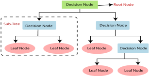
• Below diagram explains the general structure of a decision tree:

Note: A decision tree can contain categorical data (YES/NO) as well as numeric data.

Why use Decision Trees?

There are various algorithms in Machine learning, so choosing the best algorithm for the given dataset and problem is the main point to remember while creating a machine learning model. Below are the two reasons for using the Decision tree:

• Decision Trees usually mimic human thinking ability while making a decision, so it is easy to understand.
• The logic behind the decision tree can be easily understood because it shows a tree-like structure.

Decision Tree Terminologies

 Root Node: Root node is from where the decision tree starts. It represents the entire dataset, which further gets divided into two or more homogeneous sets.

 Leaf Node: Leaf nodes are the final output node, and the tree cannot be segregated further after getting a leaf node.

 Splitting: Splitting is the process of dividing the decision node/root node into sub-nodes according to the given conditions.

 Branch/Sub Tree: A tree formed by splitting the tree.

 Pruning: Pruning is the process of removing the unwanted branches from the tree.

 Parent/Child node: The root node of the tree is called the parent node, and other nodes are called the child nodes.

How does the Decision Tree algorithm Work?

In a decision tree, for predicting the class of the given dataset, the algorithm starts from the root node of the tree. This algorithm compares the values of root attribute with the record (real dataset) attribute and, based on the comparison, follows the branch and jumps to the next node.

For the next node, the algorithm again compares the attribute value with the other sub-nodes and move further. It continues the process until it reaches the leaf node of the tree. The complete process can be better understood using the below algorithm:

• Step-1: Begin the tree with the root node, says S, which contains the complete dataset.
• Step-2: Find the best attribute in the dataset using Attribute Selection Measure (ASM).
• Step-3: Divide the S into subsets that contains possible values for the best attributes.
• Step-4: Generate the decision tree node, which contains the best attribute.
• Step-5: Recursively make new decision trees using the subsets of the dataset created in step -3. Continue this process until a stage is reached where you cannot further classify the nodes and called the final node as a leaf node.

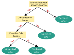
Example: Suppose there is a candidate who has a job offer and wants to decide whether he should accept the offer or not. So, to solve this problem, the decision tree starts with the root node (Salary attribute by ASM). The root node splits further into the next decision node (distance from the office) and one leaf node based on the corresponding labels. The next decision node further gets split into one decision node (Cab facility) and one leaf node. Finally, the decision node splits into two leaf nodes (Accepted offers and Declined offer). Consider the below diagram:

Attribute Selection Measures

While implementing a Decision tree, the main issue arises that how to select the best attribute for the root node and for sub-nodes. So, to solve such problems there is a technique which is called as Attribute selection measure or ASM. By this measurement, we can easily select the best attribute for the nodes of the tree. There are two popular techniques for ASM, which are:

• Information Gain
• Gini Index

1. Information Gain:

• Information gain is the measurement of changes in entropy after the segmentation of a dataset based on an attribute.
• It calculates how much information a feature provides us about a class.
• According to the value of information gain, we split the node and build the decision tree.
• A decision tree algorithm always tries to maximize the value of information gain, and a node/attribute having the highest information gain is split first. It can be calculated using the below formula:

1. Information Gain= Entropy(S)- [(Weighted Avg) *Entropy(each feature)  

Entropy: Entropy is a metric to measure the impurity in a given attribute. It specifies randomness in data. Entropy can be calculated as:

Entropy(s)= -P(yes)log2 P(yes)- P(no) log2 P(no)

Where,

• S= Total number of samples
• P(yes)= probability of yes
• P(no)= probability of no

2. Gini Index:

• Gini index is a measure of impurity or purity used while creating a decision tree in the CART(Classification and Regression Tree) algorithm.
• An attribute with the low Gini index should be preferred as compared to the high Gini index.
• It only creates binary splits, and the CART algorithm uses the Gini index to create binary splits.
• Gini index can be calculated using the below formula:

Gini Index= 1- ∑jPj2

Pruning: Getting an Optimal Decision tree

Pruning is a process of deleting the unnecessary nodes from a tree in order to get the optimal decision tree.

A too-large tree increases the risk of overfitting, and a small tree may not capture all the important features of the dataset. Therefore, a technique that decreases the size of the learning tree without reducing accuracy is known as Pruning. There are mainly two types of trees pruning technology used:

• Cost Complexity Pruning
• Reduced Error Pruning.

Advantages of the Decision Tree

• It is simple to understand as it follows the same process which a human follow while making any decision in real-life.
• It can be very useful for solving decision-related problems.
• It helps to think about all the possible outcomes for a problem.
• There is less requirement of data cleaning compared to other algorithms.

Disadvantages of the Decision Tree

• The decision tree contains lots of layers, which makes it complex.
• It may have an overfitting issue, which can be resolved using the Random Forest algorithm.
• For more class labels, the computational complexity of the decision tree may increase.

Python Implementation of Decision Tree

Now we will implement the Decision tree using Python. For this, we will use the dataset "user_data.csv," which we have used in previous classification models. By using the same dataset, we can compare the Decision tree classifier with other classification models such as KNN SVM, LogisticRegression, etc.

Steps will also remain the same, which are given below:

• Data Pre-processing step
• Fitting a Decision-Tree algorithm to the Training set
• Predicting the test result
• Test accuracy of the result(Creation of Confusion matrix)
• Visualizing the test set result.

1. Data Pre-Processing Step:

Below is the code for the pre-processing step:

1. # importing libraries  
2. Import numpy as nm  
3. Import matplotlib.pyplot as mtp  
4. Import pandas as pd  
5.  
6. #importing datasets  
7. Data_set= pd.read_csv('user_data.csv')  
8.  
9. #Extracting Independent and dependent Variable  
10. x= data_set.iloc[:, [2,3]].values  
11. y= data_set.iloc[:, 4].values  
12.  
13. # Splitting the dataset into training and test set.  
14. From sklearn.model_selection import train_test_split  
15. x_train, x_test, y_train, y_test= train_test_split(x, y, test_size= 0.25, random_state=0)  
16.  
17. #feature Scaling  
18. From sklearn.preprocessing import StandardScaler    
19. St_x= StandardScaler()  
20. x_train= st_x.fit_transform(x_train)    
21. x_test= st_x.transform(x_test)    

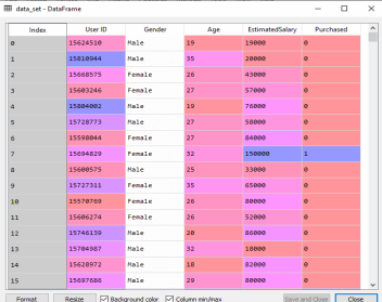
In the above code, we have pre-processed the data. Where we have loaded the dataset, which is given as:

2. Fitting a Decision-Tree algorithm to the Training set

Now we will fit the model to the training set. For this, we will import the DecisionTreeClassifier class from sklearn.tree library. Below is the code for it:

1. #Fitting Decision Tree classifier to the training set  
2. From sklearn.tree import DecisionTreeClassifier  
3. Classifier= DecisionTreeClassifier(criterion='entropy', random_state=0)  
4. Classifier.fit(x_train, y_train)  

In the above code, we have created a classifier object, in which we have passed two main parameters;

• "criterion='entropy': Criterion is used to measure the quality of split, which is calculated by information gain given by entropy.
• Random_state=0": For generating the random states.

Below is the output for this:

Out[8]:

DecisionTreeClassifier(class_weight=None, criterion='entropy', max_depth=None,

Max_features=None, max_leaf_nodes=None,

Min_impurity_decrease=0.0, min_impurity_split=None,

Min_samples_leaf=1, min_samples_split=2,

Min_weight_fraction_leaf=0.0, presort=False,

Random_state=0, splitter='best')

3. Predicting the test result

Now we will predict the test set result. We will create a new prediction vector y_pred. Below is the code for it:

1. #Predicting the test set result  
2. y_pred= classifier.predict(x_test)  

Output:

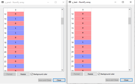
In the below output image, the predicted output and real test output are given. We can clearly see that there are some values in the prediction vector, which are different from the real vector values. These are prediction errors.

4. Test accuracy of the result (Creation of Confusion matrix)

In the above output, we have seen that there were some incorrect predictions, so if we want to know the number of correct and incorrect predictions, we need to use the confusion matrix. Below is the code for it:

1. #Creating the Confusion matrix  
2. From sklearn.metrics import confusion_matrix  
3. Cm= confusion_matrix(y_test, y_pred)  

Output:

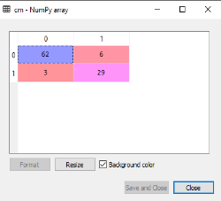
In the above output image, we can see the confusion matrix, which has 6+3= 9 incorrect predictions and62+29=91 correct predictions. Therefore, we can say that compared to other classification models, the Decision Tree classifier made a good prediction.

5. Visualizing the training set result:

Here we will visualize the training set result. To visualize the training set result we will plot a graph for the decision tree classifier. The classifier will predict yes or No for the users who have either Purchased or Not purchased the SUV car as we did in Logistic Regression. Below is the code for it:

1. #Visulaizing the trianing set result  
2. From matplotlib.colors import ListedColormap  
3. x_set, y_set = x_train, y_train  
4. x1, x2 = nm.meshgrid(nm.arange(start = x_set[:, 0].min() - 1, stop = x_set[:, 0].max() + 1, step  =0.01),  
5. Nm.arange(start = x_set[:, 1].min() - 1, stop = x_set[:, 1].max() + 1, step = 0.01))  
6. Mtp.contourf(x1, x2, classifier.predict(nm.array([x1.ravel(), x2.ravel()]).T).reshape(x1.shape),  
7. Alpha = 0.75, cmap = ListedColormap(('purple','green' )))  
8. Mtp.xlim(x1.min(), x1.max())  
9. Mtp.ylim(x2.min(), x2.max())  
10. Fori, j in enumerate(nm.unique(y_set)):  
11. Mtp.scatter(x_set[y_set == j, 0], x_set[y_set == j, 1],  
12.        c = ListedColormap(('purple', 'green'))(i), label = j)  
13. Mtp.title('Decision Tree Algorithm (Training set)')  
14. Mtp.xlabel('Age')  
15. Mtp.ylabel('Estimated Salary')  
16. Mtp.legend()  
17. Mtp.show()  

Output:

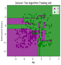
The above output is completely different from the rest classification models. It has both vertical and horizontal lines that are splitting the dataset according to the age and estimated salary variable.

As we can see, the tree is trying to capture each dataset, which is the case of overfitting.

6. Visualizing the test set result:

Visualization of test set result will be similar to the visualization of the training set except that the training set will be replaced with the test set.

1. #Visulaizing the test set result  
2. From matplotlib.colors import ListedColormap  
3. x_set, y_set = x_test, y_test  
4. x1, x2 = nm.meshgrid(nm.arange(start = x_set[:, 0].min() - 1, stop = x_set[:, 0].max() + 1, step  =0.01),  
5. Nm.arange(start = x_set[:, 1].min() - 1, stop = x_set[:, 1].max() + 1, step = 0.01))  
6. Mtp.contourf(x1, x2, classifier.predict(nm.array([x1.ravel(), x2.ravel()]).T).reshape(x1.shape),  
7. Alpha = 0.75, cmap = ListedColormap(('purple','green' )))  
8. Mtp.xlim(x1.min(), x1.max())  
9. Mtp.ylim(x2.min(), x2.max())  
10. Fori, j in enumerate(nm.unique(y_set)):  
11. Mtp.scatter(x_set[y_set == j, 0], x_set[y_set == j, 1],  
12.        c = ListedColormap(('purple', 'green'))(i), label = j)  
13. Mtp.title('Decision Tree Algorithm(Test set)')  
14. Mtp.xlabel('Age')  
15. Mtp.ylabel('Estimated Salary')  
16. Mtp.legend()  
17. Mtp.show()  

Output:

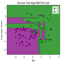
As we can see in the above image that there are some green data points within the purple region and vice versa. So, these are the incorrect predictions which we have discussed in the confusion matrix.

4.3 Statistical learning models

Statistical Learning is a set of tools for understanding data. These tools broadly come under two classes: supervised learning & unsupervised learning. Generally, supervised learning refers to predicting or estimating an output based on one or more inputs.

Unsupervised learning, on the other hand, provides a relationship or finds a pattern within the given data without a supervised output.

Let, suppose that we observe a response Y and p different predictors X = (X₁, X₂,…., Xp). In general, we can say:

Y =f(X) + ε

Here f is an unknown function, and ε is the random error term.

In essence, statistical learning refers to a set of approaches for estimating f.

In cases where we have set of X readily available, but the output Y, not so much, the error averages to zero, and we can say:

¥ = ƒ(X)

Where ƒ represents our estimate of f and ¥ represents the resulting prediction.

Hence for a set of predictors X, we can say:

E(Y — ¥)² = E[f(X) + ε — ƒ(X)]²=> E(Y — ¥)² = [f(X) - ƒ(X)]² + Var(ε)

Where,

• E(Y — ¥)² represents the expected value of the squared difference between actual and expected result.
• [f(X) — ƒ(X)]² represents the reducible error. It is reducible because we can potentially improve the accuracy of ƒ by better modeling.
• Var(ε) represents the irreducible error. It is irreducible because no matter how well we estimate ƒ, we cannot reduce the error introduced by variance in ε.

Examples of where statistical methods are used in an applied machine learning project.

1. Problem Framing: Requires the use of exploratory data analysis and data mining.
2. Data Understanding: Requires the use of summary statistics and data visualization.
3. Data Cleaning. Requires the use of outlier detection, imputation and more.
4. Data Selection. Requires the use of data sampling and feature selection methods.
5. Data Preparation. Requires the use of data transforms, scaling, encoding and much more.
6. Model Evaluation. Requires experimental design and re sampling methods.
7. Model Configuration. Requires the use of statistical hypothesis tests and
8. Estimation statistics.
9. Model Selection. Requires the use of statistical hypothesis tests and estimation statistics.
10. Model Presentation. Requires the use of estimation statistics such as confidence intervals.
11. Model Predictions. Requires the use of estimation statistics such as prediction intervals.

4.4 Learning with complete data - Naive Bayes models

Naive Bayes algorithm is a supervised learning algorithm, which is based on Bayes theorem and used for solving classification problems.It is mainly used in text classification that includes a high-dimensional training dataset.

Naive Bayes Classifier is one of the simple and most effective Classification algorithms which helps in building the fast machine learning models that can make quick predictions.

It is a probabilistic classifier, which means it predicts on the basis of the probability of an object. Some popular examples of Naive Bayes Algorithm are spam filtration, Sentimental analysis, and classifying articles.

The Naive Bayes algorithm is comprised of two words Naive and Bayes, Which can be described as:

• Naive: It is called Naive because it assumes that the occurrence of a certain feature is independent of the occurrence of other features. Such as if the fruit is identified on the bases of color, shape, and taste, then red, spherical, and sweet fruit is recognized as an apple. Hence each feature individually contributes to identify that it is an apple without depending on each other.
• Bayes: It is called Bayes because it depends on the principle of Bayes' Theorem.

Bayes' Theorem:

• Bayes' theorem is also known as Bayes' Rule or Bayes' law, which is used to determine the probability of a hypothesis with prior knowledge. It depends on the conditional probability.
• The formula for Bayes' theorem is given as:
• 

Where,

P(A|B) is Posterior probability: Probability of hypothesis A on the observed event B.

P(B|A) is Likelihood probability: Probability of the evidence given that the probability of a hypothesis is true.

P(A) is Prior Probability: Probability of hypothesis before observing the evidence.

P(B) is Marginal Probability: Probability of Evidence.

Working of Naive Bayes' Classifier:

Working of Naive Bayes' Classifier can be understood with the help of the below example:

Suppose we have a dataset of weather conditions and corresponding target variable "Play". So using this dataset we need to decide that whether we should play or not on a particular day according to the weather conditions. So to solve this problem, we need to follow the below steps:

1. Convert the given dataset into frequency tables.
2. Generate Likelihood table by finding the probabilities of given features.
3. Now, use Bayes theorem to calculate the posterior probability.

Problem: If the weather is sunny, then the Player should play or not?

Solution: To solve this, first consider the below dataset:

Frequency table for the Weather Conditions:

Applying Bayes' theorem:

P(Yes|Sunny) = P(Sunny|Yes) * P(Yes)/P(Sunny)

P(Sunny|Yes) = 3/10= 0.3

P(Sunny)= 0.35

P(Yes)=0.71

So P(Yes|Sunny) = 0.3*0.71/0.35= 0.60

P(No|Sunny) = P(Sunny|No) * P(No)/P(Sunny)

P(Sunny|NO) = 2/4=0.5

P(No)= 0.29

P(Sunny)= 0.35

So P(No|Sunny) = 0.5*0.29/0.35 = 0.41

So as we can see from the above calculation that P(Yes|Sunny)>P(No|Sunny)

Advantages of Naive Bayes Classifier.

• Naive Bayes is one of the fast and easy ML algorithms to predict a class of datasets.
• It can be used for Binary as well as Multi-class Classifications.
• It performs well in Multi-class predictions as compared to the other Algorithms.
• It is the most popular choice for text classification problems.

Disadvantages of Naive Bayes Classifier.

• Naive Bayes assumes that all features are independent or unrelated, so it cannot learn the relationship between features.

Types of Naive Bayes Model.

There are three types of Naive Bayes Model, which are given below.

• Gaussian: The Gaussian model assumes that features follow a normal distribution. This means if predictors take continuous values instead of discrete, then the model assumes that these values are sampled from the Gaussian distribution.
• Multinomial: The Multinomial Naive Bayes classifier is used when the data is multinomial distributed. It is primarily used for document classification problems, it means a particular document belongs to which category such as Sports, Politics, education, etc.
  The classifier uses the frequency of words for the predictors.
• Bernoulli: The Bernoulli classifier works similar to the Multinomial classifier, but the predictor variables are the independent Booleans variables. Such as if a particular word is present or not in a document. This model is also famous for document classification tasks.

4.5 Learning with hidden data – EM algorithm

Many real world problems have hidden variables (or) latent variables which are not observable in the data that are available for learning.

For Example: Medical record often include the observed symptoms, treatment applied and outcome of the treatment, but seldom contain a direct observation of disease itself.

Assumed the diagnostic model for heart disease.

There are three observable predisposing factors and 3 observable symptoms. Each variable has 3 possible values (none, moderate and severe)

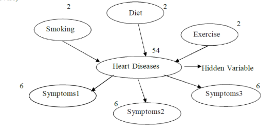
If hidden is removed the total number of parameters increases from 78 (54 + 2 + 2 + 2 + 6 + 6 + 6) to 708

Hidden variables can dramatically reduce the number of parameters required to specify the

Bayesian network, thereby reduce the amount of data needed to learn the parameters.

It also includes estimating probabilities when some of the data are missing.

The reason we learn Bayesian network with hidden variable is that it reveals interesting structures in our data.

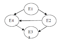
Consider a situation in which you can observe a whole bunch of different evidence variables, Er through En. They are all different symptoms that a patient might have.

Different systems

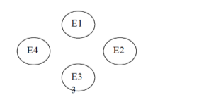
If the variables are conditionally dependent on one another. We will get a highly connected graph that representing the entire joint distribution between the variables.

The model can be simpler by introducing an additional cause node. It represents the underlying disease state that was causing the patient symptoms.

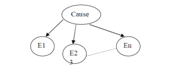
This will parameters, because the evident variables are conditionally independent given the causes.

The model cab be simpler by introducing an additional cause node. It represents the underlying disease state that was causing the patient symptoms.

Missing data

Imagine that we have 2 binary variables A and B that are not independent. We try to estimate the Joint distribution.

It is done by counting how many were (true, true) and how may (false, false) and divide by the total number of cases to get maximum likelihood estimate.

The above data set has some data missing (denoted on “H”). There’s no real way to guess the value during our estimation problem.

The missing data items can be independent of the value it would have had. The data can be missed if there is a fault in the instrument used to measure.

For Example: Blood pressure instrument fault, so blood pressure data can be missing)

EM Algorithm

a. Want to find θ to maximize PR(D/ θ)

To find theta (θ) that maximizes the probability of data for given theta (θ)

b. Instead find θ, to maximize, where tilde

log

Where Probability distribution over hidden variables, H=Hidden Variables

c. Find Optimum value for g

• Holding θ fixed and optimizing
• Holding fixed and optimizing θ
• And repeat the procedure over and over again

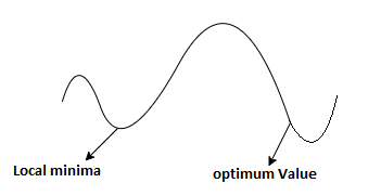
d. g has some local and global optima as PR(D/θ)

e. Example

i. Pick initial

Ii. Probability of hidden variables giventhe observed data and the current model.

Loop until it converges

We find the maximum likelihood model for  the “expected data ” using the distribution over H to generate expected counts for different case.

Iii. Increasing likelihood.

Iv.   Convergence is determined (but difficult)

v.     Process with local optima i.e., sometime it converges quite effectively to the maximum model that’s near the one it started with, but there’s much better model somewhere else in the space.

4.6 Reinforcement learning

Reinforcement is feedback from which the agent comes to know that something good has happened when it wins and that something bad has happened when it loses. This is also called as reward.

For Example:

In chess game, the reinforcement is received only at the end of the game.

In ping-pong, each point scored can be considered a reward; when learning to crawl, any forward motion is an achievement.

The framework for agents regards the reward as part of the input percept, but the agent must be hardwired to recognize that part as a reward rather than as just another sensory input.

Rewards served to define optimal policies in Markov decision processes.

An optimal policy is a policy that maximizes the expected total reward.

The task of reinforcement learning is to use observed rewards to learn an optimal policy for the environment.

Learning from these inforcements or rewards is known as reinforcement learning

In reinforcement learning an agent is placed in an environment, the following are the agents

1. Utility-based agent
2. Q-Learning agent
3. Reflex agent

The following are the Types of Reinforcement Learning.

Passive Reinforcement Learning

In this learning, the agent’s policy is fixed and the task is to learn the utilities of states.

• It could also involve learning a model of the environment.
• In passive learning, the agent’s policy is fixed(i.e.) in state s, it always executes the action
• Its goal is simply to learn the utility function
• For example: Consider the 4×3 world.
• The following table shows the policy for that world.

• The following table shows the corresponding utilities

• Clearly, the passive learning task is similar to the policy evaluation task.
• The main difference is that the passive learning agent does not know
• Neither the transistion model T(s,a,s*), which specifies the probability of reaching state’s from state’s after doing action a:
• Nor does it know the reward function R(s), which specifies the reward for each state.
• The agent executes a set of trials in the environment using its policy
• In each trial, the agent starts in state (1,1) and experiences a sequence of state transitions until it reaches one of the terminal states (4,2) or (4,3)
• Its percepts supply both current state and the reward received in thea state.
• Typical trials might look like this:

• Note that each state percept is subscripted with the reward received.
• The object is to use the information about rewards to learn the expected utility associated with each nonterminal state s.
• The utility is defined ot be the expected sum of (discounted rewards obtained if policy is followed, the utility function is written as
• 
• For the 4×3 world set =1

Active Reinforcement Learning

• A passive learning agent has a fixed policy that determine its behaviour
• “An active agent must decide what actions to do”
• An ADP agent can be taken an considered how it must be modified to handle this new freedom.
• The following are the required modifications:

• First the agent will need to learn a complete model with outcome probabilities for an actions. The simple learning mechanism used by PASSIVE-ADP-AGENT will do just fine for this.
• Next, take into account the fact that  the agent has a choice of actions. The utilities it needs to learn are those defined by the optimal policy.             

• These equations can be solved to obtain the utility function U using he value iteration or policy algorithms.
• Having obtained a utility fucntion U that is optimal for the learned model, the agent can extract an optimal action by one-step look ahead to maximize the expected utility;
• Alternatively, if it uses policy iteration, the optimal policy is already available, so it should simply execute the action the optimal policy recommends.

References:

1. Stuart Russell, Peter Norvig, “Artificial Intelligence – A Modern Approach”, Pearson Education

2. Elaine Rich and Kevin Knight, “Artificial Intelligence”, McGraw-Hill

3. E Charniak and D McDermott, “Introduction to Artificial Intelligence”, Pearson Education

4. Dan W. Patterson, “Artificial Intelligence and Expert Systems”, Prentice Hall of India