Unit - 5

Pattern Recognition

5.1 Introduction

Pattern recognition is a branch of machine learning that focuses on the recognition of patterns and regularities in data,

It is the study of how machines can observe the environment intelligently, learn to distinguish patterns of interest from their backgrounds and make reasonable & correct decisions about the different classes of objects.

Patterns may be a finger print image, handwritten cursive word, a human face, iris of human eye or a speech signal.

These examples are called input stimuli. Recognition establishes a close match between some new stimulus and previously stored stimulus patterns.

Pattern recognition systems are in many cases trained from labelled "training" data That is supervised learning, but when no labelled data are available other algorithms can be used to discover previously unknown patterns i.e., unsupervised learning

At the most abstract level patterns can also be some ideas, concepts, thoughts, procedures Activated in human brain and body. This is known as the study of human psychology. 

Examples are Speech recognition, speaker identification and automatic medical diagnosis. 

In a typical pattern recognition application, the raw data is processed and converted into a form that is amenable for a machine to use.

Pattern recognition has classification and cluster of patterns. 

1. In classification an appropriate class label is assigned to a pattern based on an abstraction that is generated using a set of training patterns or domain knowledge. Classification is used in supervised learning.
2. Clustering generated a partition of the data which helps decision making, the specific decision-making activity of interest to us. Clustering is used in an unsupervised learning.

Pattern recognition features: 

1. Pattern recognition system should recognize familiar pattern quickly and accurate
2. Recognize and classify unfamiliar objects
3. Accurately recognize shapes and objects from different angles
4. Identify patterns and objects even when partly hidden
5. Recognize patterns quickly with ease, and with automaticity.

Training and Learning in Pattern Recognition 

Learning is a phenomenon through which a system gets trained and becomes adaptable to give result in an accurate manner. Learning is the most important phase as how well the system performs on the data provided to the system depends on which algorithms used on the data.

What is Training and Testing

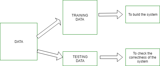
The system is trained using a finite set of patterns- the training set.

If the correct classification for these patterns is known then this is Supervised

Learning, otherwise it is Unsupervised Learning.

The system is evaluated using a different set of patterns - the test set.

5.2 Design principles of pattern recognition system

The two main types are

1. Statistical Pattern Recognition 2. Syntactic Pattern Recognition

1. Of the two, the statistical pattern recognition has been more popular and received a major attention in the literature.
2. The main reason for this is that most of the practical problems in this area have to deal with noisy data and uncertainty and statistics and probability are good tools to deal with such problems.
3. On the other hand, formal language theory provides the background for syntactic pattern recognition. Systems based on such linguistic tools, more often than not, are not ideally suited to deal with noisy environments. However, they are powerful in dealing with well-structured domains. Also, recently there is a growing interest in statistical pattern recognition because of the influence of statistical learning theory.
4. This naturally prompts us to orient material in this course towards statistical classification and clustering. Statistical Pattern Recognition
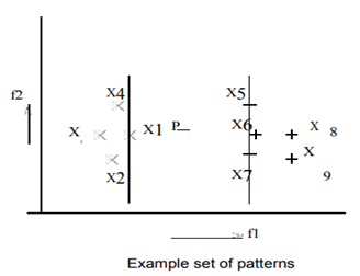
5. In statistical pattern recognition, we use vectors to represent patterns and class labels from a label set.
6. The abstractions typically deal with probability density/distributions of points in multi-dimensional spaces, trees and graphs, rules, and vectors themselves.
7. Because of the vector space representation, it is meaningful to talk of subspaces/projections and similarity between points in terms of distance measures.
8. There are several soft computing tools associated with this notion. Soft computing techniques are tolerant of imprecision, uncertainty and approximation. These tools include neural networks, fuzzy systems and evolutionary computation.
9. For example, vectorial representation of points and classes are also employed by neural networks, fuzzy set and rough set-based pattern recognition schemes. • In pattern recognition, we assign labels to patterns. This is achieved using a set of semantically labelled patterns; such a set is called the training data set. It is obtained in practice based on inputs from experts.

Comparison Between Statistical Approach and Structural Approach.

5.3 Statistical Pattern recognition

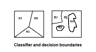
1. Statistical classification problem, there is a decision boundary is a hyper surface that partitions the underlying vector space into two sets. A decision boundary is the region of a problem space in which the output label of a classifier is ambiguous.

Classifier is a hypothesis/ discrete valued function that is used to assign       class labels to particular data points.

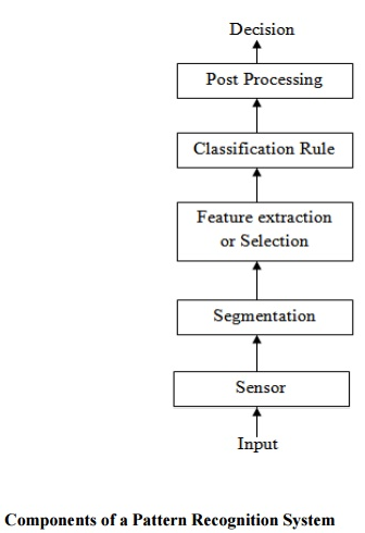
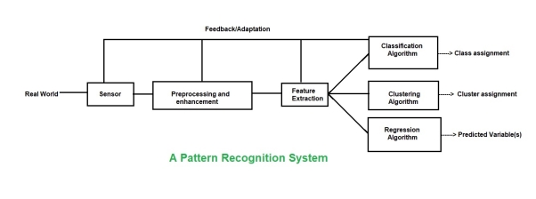
Pattern recognition system consists of-

5.4 Parameter estimation methods - Principle Component Analysis (PCA) and Linear Discriminant Analysis (LDA)

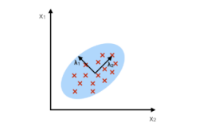
This is a mathematical procedure that uses orthogonal transforms to convert a set of Observations of possibly correlated variables into a set of linearly uncorrelated variables known as Principal Components. So here we preserve the most variance with reduced dimensions and minimum mean square error.

Number of principal components are less than or equal to number of original variables.

First Principal component has largest variance. Successively it decreases.

These are defined by Best Eigen Vectors of Covariance Matrix of vector X.

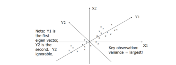
Geometrical analysis of PCA

i. PCA projects data along directions where 𝜎 square is maximum.

Ii. These directions are determined by eigen vectors of covariance matrix corresponding to largest

Eigen values.

Iii. Magnitude of variance is variance of data along the directions of eigen values.

Iv. Eigen Values are characteristic values given as AX = 𝜆 𝑋, A is m x n matrix, 𝜆 𝑖𝑠 𝑒𝑖𝑔𝑒𝑛 𝑣𝑎𝑙𝑢𝑒

PCA: Component axes that maximize the variance

• Degree to which the variables are linearly correlated is represented by their covariance.
• PCA uses Euclidean Distance calculated from the p variables as the measure of dissimilarity among the n objects The eigen values (latent roots) of S are solutions  to the characteristic equation

• The eigen values are the variances of the coordinates on each principal component axis. Coordinates of each object on the kth principal axis, known as the scores on PC, k are computed s mentioned below.

Steps of PCA

• Let  be the mean vector (taking the mean of all rows)
• Adjust the original data by the mean
• Compute the covariance matrix C of adjusted X
• Find the eigen vectors and eigen values of C.
• For matrix C, vectors e (=column vector) having same direction as Ce:
• Eigenvectors of C is e such that Ce=e
•  is called an eigen value of C. Ce=e

Applications of PCA

1. Face recognition
2. Image compression
3. Gene expression analysis

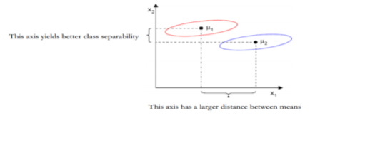
LDA is to perform dimensionality reduction while preserving as much of the class discrimination information as possible. Here in LDA data is projected from d – dimensions onto a line. If the samples formed well separated compact clusters in d- space then projection onto an arbitrary line will usually produce poor recognition performance. By rotating the line, we can find an orientation for which projected samples are well separated.

• Assume we have m-dimensional samples of which belong to and .
• We seek to obtain a scalar y by projecting the samples x onto a line (C-1 space, C=2)

where and

Where w is the projection vectors used to project x to y.

• Of all the possible lines we would like to select the one that maximizes the reparability of the scalars.

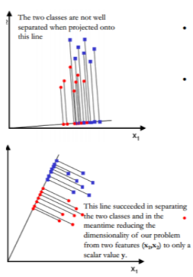
• The mean vector of each class in x and y feature space is-

and

projecting x to y will lead to projecting the mean of x to the mean of y.

• We could then choose the distance between the projected means as our objective function
• 

PCA   and LDA Common features.

1. Both list the current axes in order of significance.
2. PC1 accounts for the most significant data variance, PC2 does the second best job, and so on.
3. LD1 accounts for the most significant data variance, LD2 does the second best job, and so on.
4. The algorithms tell us which attribute or function contributes more to the development of the new axes.
5. LDA is same as PCA, each attempting to decrease the measurements.
6. For the most variation, PCA searches for attributes.
7. LDA seeks to optimize the differentiation of groups that are identified.

Note- The main difference is that LDA takes into class labels into account, where PCA is unsupervised and does not.

5.5 Classification Techniques – Nearest Neighbor (NN) Rule

KNN Algorithm

1. It is one of the simplest Machine Learning algorithms based on Supervised Learning technique.
2. Algorithm assumes the similarity between the new case/data and available cases, puts the new case into the category that is most similar to the available categories.
3. Algorithm stores all the available data and classifies a new data point based on the similarity. This means when new data appears then it can be easily classified into a well suite category by using K NN algorithm.
4. Algorithm can be used for Regression and Classification but mostly it is used for the Classification type problems.
5. It is a non-parametric algorithm, which means it does not make any assumption on underlying data.
6. It is known as lazy learner algorithm because it does not learn from the training set immediately instead it stores the dataset and at the time of classification, it performs an action on the dataset.
7. Algorithm at the training phase just stores the dataset and when it gets new data, then it classifies that data into a category that is much similar to the new data.

Importance of KNN Algorithm

Consider there are 2 categories, that is Category A and Category B, and we have a new data point x1, so this data point will lie in which of these categories. To solve this type of problem, we need algorithm. With the help of algorithm, we can easily identify the category or class of a particular dataset. Consider the below diagram.

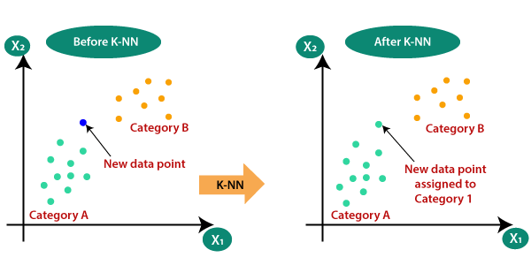
The K-NN working can be explained on the basis of the below algorithm.

1. Step-1: Select the number K of the neighbors
2. Step-2: Calculate the Euclidean distance of K number of neighbors
3. Step-3: Take the K nearest neighbors as per the calculated Euclidean distance.
4. Step-4: Among these k neighbors, count the number of the data points in each category.
5. Step-5: Assign the new data points to that category for which the number of the neighbor is maximum.
6. Step-6: Our model is ready.

5.6 Bayes Classifier

Classification using Bayes Decision Theory

•  This approach classification is carried out using probabilities of classes.

• It is assumed that we know the a priori or the prior probability of each class. If we have two classes C1 and C2, then the prior probability for class C1 is PC 1 and the prior probability for class C2 is PC 2.

• If the prior probability is not known, the classes are taken to be equally likely.

• If prior probability is not known and there are two classes C1 and V2, then it is assumed PC 1 = PC 2 = 0.5.

• If PC 1 and PC 2 are known, then when a new pattern x comes along, we need to calculate P (C1|x) and P (C2|x).

• The bayes theorem is used to compute P (C1|x) and P (C2|x).

• Then if P (C1|x) P (C1|x) < P (C2 decision rule.

Bayes Rule

• P (C2|x), the pattern is assigned to Class 1 and if (C2|x), it is assigned to Class 2. This is called the Bayes

• If P (Ci) is the prior probability of Class i, and P (X |Ci) is the conditional density of X given class Ci, then a posterior probability of Ci is given by   P (X |C) P (C) P Ci X (i) iP X

• Bayes theorem provides a way of calculating the posterior probability P (Ci| X). In other words, after observing X, the posterior probability that the class is ci can be calculated from Bayes theorem. It is useful to convert prior probabilities to posterior probabilities.

• P (X) is given by P (X) = i P (X | Ci) P (Ci)

• Let the probability that an elephant is black be 80% and that an elephant is white be 20%. This means P (elephant is black) = 0.8 and P (elephant is white) =0.2. With only this information, any elephant will be classified as being black. This is because the probability of error in this case is only 0.2 as opposed to classifying the elephant as white

Which results in a probability of error of 0.8. When additional information is available, it can be used along with the information above.

If we have probability that elephant belongs to region X is 0.2. Now if the elephant belongs to region X, we need to calculate the posterior probability that the elephant is white. i.e., P (elephant is white | elephant belongs to region) or P (W | X). This can be calculated by using Bayes theorem. If 95% of the time when the elephant is white, it is because it belongs to the region X. Then

P (W | X) = P (X |W) ∗ P (W) = 0.95∗ 0.2 = 0.95P (X) 0.2

The probability of error is 0.05 which is the probability that the elephant is not white given that it belongs to region X.

Minimum Error Rate Classifier

• If it is required to classify a pattern X, then the minimum error rate classifier classifies the pattern X to the class C which has the maximum posterior probability P (C | X).

• If the test pattern X is classified as belonging to Class C, then the error in the classification will be (1 - P (C | X)).

• It is evident to reduce the error, X has to be classified as belonging to the class for which P (C | X) is maximum.

• The expected probability of error is given by

(1 − P (C |X)) P (X) dX

X to the power is above value

This is minimum when P (C | X) is maximum (for a specified value of (X).

Naive Bayes Classifier

• A naive bayes classifier is based on applying Bayes theorem to find the class of a pattern.

• The assumption made here is that every feature is class conditionally independent.

• Due to this assumption, the probabilistic classifier is simple.

• In other words, it is assumed that the effect of each feature on a given class is independent of the value of other features.

• Since this simplifies the computation, though it may not be always true, it is considered to be a naive classifier.

80

• Even though this assumption is made, the Naive Bayes Classifier is found to give results comparable in

Performance to other classifiers like neural network classifiers and classification trees.

• Since the calculations are simple, this classifier can be used for large databases where the results are obtained fast with reasonable accuracy.

• Using the minimum error rate classifier, we classify the pattern X to the class with the maximum posterior probability P (c | X). In the naive bayes classifier, this can be written as Working of Naive Bayes' Classifier.

where are the features.

Using Bayes theorem, this can be written as

Since every feature is independent of every other feature , for , given the class

So, we get,

The conditional distribution over the class variable C is

Where Z is a scaling factor.

The Naïve Bayes classification uses only the prior probabilities of classes P(C) and the independent probability distributions

Parameter Estimation

In supervised learning, training set is given. Using the training set, all the parameters of the bayes model can be computed.

If of the training examples out of n belong to Class C, then the prior probability of Class C will be

• In a class C, if samples take a range of values (or a single value) out of a total of samples in the class, then the prior probability of the feature being in this range in this class will be

In case of the feature taking a small number of integer values, this can be calculated for each of these values. For example, it would be

If of the patterns of Class c take on the value 6.

Let us estimate the parameters for a training set which has 00 patterns of Class 1, 90 patterns of Class 2, 140 patterns of Class 3 and 100 patterns of Class 4 the prior probability of each class can be calculated.

The prior probability of Class 1 is

The prior probability of Class 2 is

The prior probability of Class 3 is

The prior probability of Class 4 is

Out pf the 100 examples of Class 1, if we consider a particular feature f1 and 25 take on the value 2, then the prior probability that in class 1 the feature f1 is 0 is

The prior probability that in class 1 the feature f1 is 1 is

The prior probability that in class 1 the feature f1 is 2 is

Advantages of NB Classifier.

• NB is one of the fast and easy ML algorithms to predict a class of datasets.
• It can be used for Binary as well as Multi-class Classifications.
• It performs well in multi-class predictions as compared to the other Algorithms.
• It is the most popular choice for text classification problems.

Disadvantages of NB Classifier.

• NB assumes that all features are independent or unrelated, so it cannot learn the relationship between features.

Types of NB Model.

• Gaussian: The Gaussian model assumes that features follow a normal distribution. This means if predictors take continuous values instead of discrete, then the model assumes that these values are sampled from the Gaussian distribution.
• Multinomial: The Multinomial NB classifier is used when the data is multinomial distributed. It is primarily used for document classification problems, it means a particular document belongs to which category such as Sports, Politics, education, etc.
• Bernoulli: The Bernoulli classifier works similar to the Multinomial classifier, but the predictor variables are the independent Booleans variables. Such as if a particular word is present or not in a document. This model is also famous for document classification tasks.

5.7 Support Vector Machine (SVM)

Support Vector Machines: This is a linear machine with a case of separable patterns that may arise in the context of pattern classification. Idea is to construct a HYPERPLANE as a direction surface in such a way that the margin of separation between positive and negative examples is maximized.

A good example of such a system is classifying a set of new documents into positive or negative sentiment groups, based on other documents which have already been classified as positive or negative. Similarly, we could classify new emails into spam or non-spam, based on a large corpus of documents that have already been marked as spam or non-spam by humans.

SVMs are highly applicable to such situations.

1. SVM is an approximate implementation of Structural Risk Minimization.
2. Error rate of a machine on test data is bounded by the sum of training error rate and term that depends on Vapnik Chervonenki’s dimension.
3. SVM sets first term to zero and minimizes second term. We use SVM learning algorithm to construct following three types of learning machines:

(i) Polynomial learning machine

(ii) Two layer perceptron’s

(iii) Radial basis function N/W

Condition is as: Test error rate ≤ Train error rate + f (N, h, p).

Where N: Size of training set, h: Measure of model complexity P: Probability that this bound fails. If we consider an element of our p-dimensional feature space, i.e. →x= (x1,...,xp)∈Rp, then we can mathematically define an affine Hyper plane by the following equation: b0+b1x1+...+bpxp=0,

b0≠0 gives us an affine plane (i.e., it does not pass through the origin). We can use a more succinct notation for this equation by introducing the summation sign: b0+p∑ j=1bj xj=0.

The line that maximizes the minimum margin is better. Maximum margin separator is determined by a subset of data points. Data points in the subset are called Support Vectors. Support vectors are used to decide which side of separator a test case is ON.

Consider a training set {(𝑿𝒊, 𝒅𝒊,)} for i= 1 to n, where Xi is input pattern for ith example.

And di is the desired response (Target output). Let 𝒅𝒊, = +𝟏 and 𝒅𝒊, = −𝟏 Pattern classes for positive and negative examples are linearly separable. Hyper Plane decision surface is given as below equation:

𝑾𝑻 X + b = 0, then di =0(when data point is on the line)

Where W: adjustable weight factor and b is Bias.

Therefore, 𝑾𝑻 Xi + bi ≥ 𝟎 for 𝒅𝒊, = +𝟏 and 𝑾𝑻 Xi + bi < 𝟎 for 𝒅𝒊, = −𝟏.

Closest data point is called Margin of Separation. Denoted by ρ. Objective of SVM is to maximize ρ for Optimal Hyper plane.

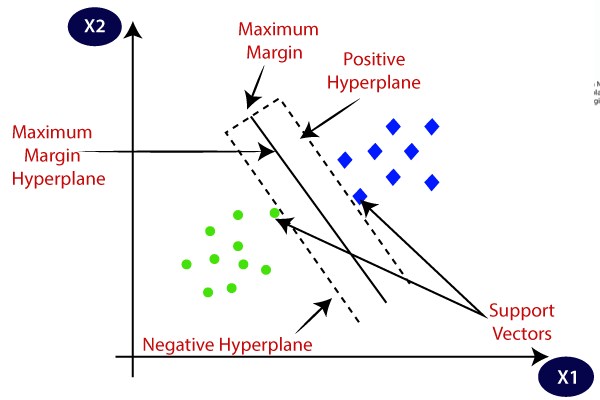
SVM can be of two types.

1. Linear SVM: Linear SVM is used for linearly separable data, which means if a dataset can be classified into two classes by using a single straight line, then such data is termed as linearly separable data, and classifier is used called as Linear SVM classifier.
2. Non linear SVM: Non Linear SVM is used for non-linearly separated data, which means if a dataset cannot be classified by using a straight line, then such data is termed as non linear data and classifier used is called as Non-linear SVM classifier.

Linear SVM

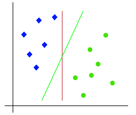
The working of the SVM algorithm can be understood by using an example. Suppose we have a dataset that has two tags (green and blue), and the dataset has two features x1 and x2. We want a classifier that can classify the pair (x1, x2) of coordinates in either green or blue. Consider the below image.

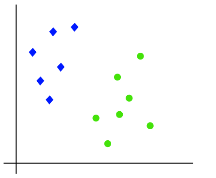
So, as it is 2-d space so by just using a straight line, we can easily separate these two classes. But there can be multiple lines that can separate these classes. Consider the below image.

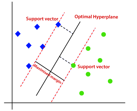
Hence, the SVM algorithm helps to find the best line or decision boundary; this best boundary or region is called as a hyperplane. SVM algorithm finds the closest point of the lines from both the classes. These points are called support vectors. The distance between the vectors and the hyperplane is called as margin. And the goal of SVM is to maximize this margin. The hyperplane with maximum margin is called the optimal hyperplane.

Non-Linear SVM

If data is linearly arranged, then we can separate it by using a straight line, but for non-linear data, we cannot draw a single straight line. Consider the below image.

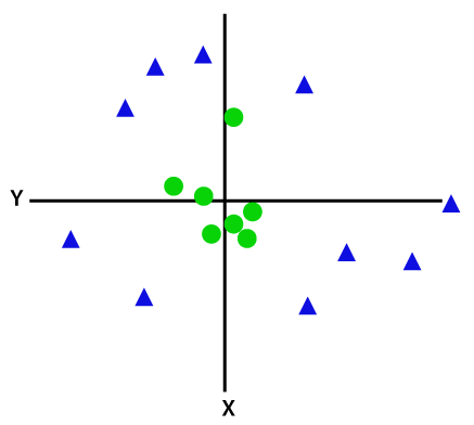
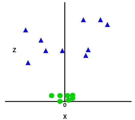
So, to separate these data points, we need to add one more dimension. For linear data, we have used two dimensions x and y, so for non-linear data, we will add a third-dimension z. It can be calculated as.

z=x2 +y2

By adding the third dimension, the sample space will become as below image.

5.8 K – means clustering

K –Nearest Neighbor Estimation:

1. Calculate “d (x, xi)” i =1, 2,….., n; where d denotes the Euclidean distance between the

Points.

2. Arrange the calculated n Euclidean distances in non-decreasing order.

3. Let k be a +ve integer, take the first k distances from this sorted list.

4. Find those k-points corresponding to these k-distances.

5. Let ki denotes the number of points belonging to the ith class among k points i.e., k ≥ 0

6. If ki >kj ∀ i ≠ j then put x in class i.

Advantages of KNN

1. Easy to understand

2. No assumptions about data

3. Can be applied to both classification and regression

4. Works easily on multi-class problems

Disadvantages are

1. Memory Intensive / Computationally expensive

2. Sensitive to scale of data

3. Not work well on rare event (skewed) target variable

4. Struggle when high number of independent variables

To measure the quality of clustering ability of any partitioned data set, criterion function is used.

1. Consider a set, B = { x1,x2,x3…xn} containing “n” samples, that is partitioned exactly into “t”

Disjoint subsets i.e. B1, B2,…..,Bt.

2. The main highlight of these subsets is, every individual subset represents a cluster.

3. Sample inside the cluster will be similar to each other and dissimilar to samples in other clusters.

4. To make this possible, criterion functions are used according the occurred situations.

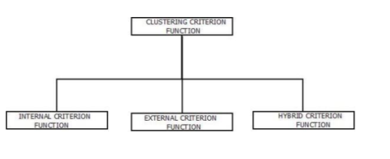
Internal Criterion Function

a) It is an intra-cluster view.

b) It optimizes a function and measures the quality of clustering ability various clusters which are different from each other.

External Criterion Function

a) It is an inter-class view.

b) It optimizes a function and measures the quality of clustering ability of various clusters which are different from each other.

Hybrid Criterion Function

a) It is used as it has the ability to simultaneously optimize multiple individual Criterion Functions unlike as Internal Criterion Function and External Criterion Function

References:

1. Stuart Russell, Peter Norvig, “Artificial Intelligence – A Modern Approach”, Pearson Education

2. Elaine Rich and Kevin Knight, “Artificial Intelligence”, McGraw-Hill

3. E Charniak and D McDermott, “Introduction to Artificial Intelligence”, Pearson Education

4. Dan W. Patterson, “Artificial Intelligence and Expert Systems”, Prentice Hall of India