1.1 Basic Terminology

The building blocks of every program or software are data structures. The most challenging challenge for a programmer is deciding on a suitable data structure for a program. When it comes to data structures, the following terminology is utilized.

Data: The data on a student can be defined as an elementary value or a set of values, for example, the student's name and id.

Group items: Group items are data items that include subordinate data items, such as a student's name, which can have both a first and a last name.

Record: A record can be characterized as a collection of several data objects. For example, if we consider the student entity, the name, address, course, and grades can all be gathered together to constitute the student's record.

File: A file is a collection of various records of one type of entity; for example, if there are 60 employees in the class, the relevant file will contain 20 records, each containing information about each employee.

Attribute and Entity: A class of objects is represented by an entity. It has a number of characteristics. Each attribute represents an entity's specific property.

1.2 Elementary Data Organization

Linear data structure - In Data structure is linear. The processing of data items can be done in a linear fashion, that is, one by one. A linear structure is a data structure that can hold a large number of objects. The things can be added in a variety of ways, but once added, they maintain a constant relationship with their neighbors. For example, a collection of numbers, a collection of strings, and so on.

Once an item is added, it remains in its current location in relation to the things that came before and after it. Array, Linked list, Stack, and Queue are examples of linear data structures.

Non - linear data structure - The processing of data items in a non-linear data structure is not linear. Graphs and trees are examples of non-linear data structures.

1.3 Built in Data Types in C

A data type is assigned to each variable in C. Each data type necessitates a particular amount of memory and can be used in a variety of ways. Let's take a look at each one individually.

The examples below show some of the most common data types used in C:

Char - In C, this is the simplest data type. In virtually all compilers, it stores a single character and only uses one byte of memory.

Int - Int variables are used to store integers, as their name implies.

Float - It's used to hold single-precision decimal integers (numbers with a floating-point value).

Double - It's used to hold decimal integers with double precision (numbers with floating point values).

Distinct data formats have different number ranges that they can store. These ranges may differ from one compiler to the next. On a 32-bit gcc compiler, the ranges are listed below, along with the RAM requirements and format specifiers.

Key takeaway

1.4 Algorithm

What is an Algorithm?

An algorithm is a process or a set of rules required to perform calculations or some other problem-solving operations especially by a computer. The formal definition of an algorithm is that it contains the finite set of instructions which are being carried in a specific order to perform the specific task. It is not the complete program or code; it is just a solution (logic) of a problem, which can be represented either as an informal description using a Flowchart or Pseudocode.

Characteristics of an Algorithm

The following are the characteristics of an algorithm:

●      Input: An algorithm has some input values. We can pass 0 or some input value to an algorithm.

●      Output: We will get 1 or more output at the end of an algorithm.

●      Unambiguity: An algorithm should be unambiguous which means that the instructions in an algorithm should be clear and simple.

●      Finiteness: An algorithm should have finiteness. Here, finiteness means that the algorithm should contain a limited number of instructions, i.e., the instructions should be countable.

●      Effectiveness: An algorithm should be effective as each instruction in an algorithm affects the overall process.

●      Language independent: An algorithm must be language-independent so that the instructions in an algorithm can be implemented in any of the languages with the same output.

Dataflow of an Algorithm

●      Problem: A problem can be a real-world problem or any instance from the real-world problem for which we need to create a program or the set of instructions. The set of instructions is known as an algorithm.

●      Algorithm: An algorithm will be designed for a problem which is a step by step procedure.

●      Input: After designing an algorithm, the required and the desired inputs are provided to the algorithm.

●      Processing unit: The input will be given to the processing unit, and the processing unit will produce the desired output.

●      Output: The output is the outcome or the result of the program.

Why do we need Algorithms?

We need algorithms because of the following reasons:

●      Scalability: It helps us to understand scalability. When we have a big real-world problem, we need to scale it down into small-small steps to easily analyze the problem.

●      Performance: The real-world is not easily broken down into smaller steps. If the problem can be easily broken into smaller steps means that the problem is feasible.

Let's understand the algorithm through a real-world example. Suppose we want to make a lemon juice, so following are the steps required to make a lemon juice:

Step 1: First, we will cut the lemon into half.

Step 2: Squeeze the lemon as much as you can and take out its juice in a container.

Step 3: Add two tablespoons of sugar in it.

Step 4: Stir the container until the sugar gets dissolved.

Step 5: When sugar gets dissolved, add some water and ice in it.

Step 6: Store the juice in a fridge for 5 to minutes.

Step 7: Now, it's ready to drink.

The above real-world can be directly compared to the definition of the algorithm. We cannot perform step 3 before step 2, we need to follow the specific order to make lemon juice. An algorithm also says that each and every instruction should be followed in a specific order to perform a specific task.

Now we will look at an example of an algorithm in programming.

We will write an algorithm to add two numbers entered by the user.

The following are the steps required to add two numbers entered by the user:

Step 1: Start

Step 2: Declare three variables a, b, and sum.

Step 3: Enter the values of a and b.

Step 4: Add the values of a and b and store the result in the sum variable, i.e., sum=a+b.

Step 5: Print sum

Step 6: Stop

Key takeaway

1.5 Efficiency of an Algorithm

Following are the conditions where we can analyze the algorithm:

●      Time efficiency: - indicates how fast algorithm is running

●      Space efficiency: - how much extra memory the algorithm needs to complete its execution

●      Simplicity: - generating sequences of instruction which are easy to understand.

●      Generality: - It fixes the range of inputs it can accept. The generality of problems which algorithms can solve.

The time efficiencies of a large number of algorithms fall into only a few classes

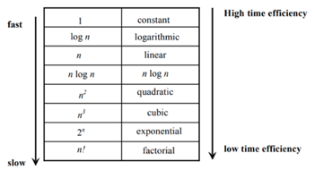
Fig 1: time efficiency

1.6 Time and Space Complexity

Time complexity: The time complexity of an algorithm is the amount of time required to complete the execution. The time complexity of an algorithm is denoted by the big O notation. Here, big O notation is the asymptotic notation to represent the time complexity. The time complexity is mainly calculated by counting the number of steps to finish the execution.

Let's understand the time complexity through an example.

In the above code, the time complexity of the loop statement will be at least n, and if the value of n increases, then the time complexity also increases. While the complexity of the code, i.e., return sum will be constant as its value is not dependent on the value of n and will provide the result in one step only. We generally consider the worst-time complexity as it is the maximum time taken for any given input size.

Space complexity: An algorithm's space complexity is the amount of space required to solve a problem and produce an output. Similar to the time complexity, space complexity is also expressed in big O notation.

For an algorithm, the space is required for the following purposes:

To track the function calls, jumping statements, etc.

Key takeaway

1.7 Asymptotic notations: Big Oh, Big Theta and Big Omega

Big Oh (O) Notation:

● It is the formal way to express the time complexity.

● It is used to define the upper bound of an algorithm’s running time.

● It shows the worst-case time complexity or largest amount of time taken by the algorithm to perform a certain task.

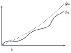
Fig 2: Big Oh notation

Here, f (n) <= g (n) ……………. (eq1)

Where n>= k, C>0 and k>=1

If any algorithm satisfies the eq1 condition then it becomes f (n)= O (g (n))

Big Omega (ῼ) Notation

● It is the formal way to express the time complexity.

● It is used to define the lower bound of an algorithm’s running time.

● It shows the best-case time complexity or best of time taken by the algorithm to perform a certain task.

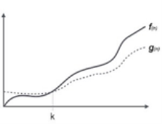
Fig 3: Big omega notation

Here, f (n) >= g (n)

Where n>=k and c>0, k>=1

If any algorithm satisfies the eq1 condition then it becomes f (n)= ῼ (g (n))

Theta (Θ) Notation

● It is the formal way to express the time complexity.

● It is used to define the lower as well as upper bound of an algorithm’s running time.

● It shows the average case time complexity or average of time taken by the algorithm to perform a certain task.

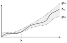
Fig 4: Theta notation

Let C1 g(n) be upper bound and C2 g(n) be lower bound.

C1 g(n)<= f (n)<=C2 g(n)

Where C1, C2>0 and n>=k

Key takeaway

1.8 Time-Space trade-off

● Two Space-for-Time Algorithm Varieties:

● Input enhancement - To store some info, preprocess the input (or its portion) to be used in solving the issue later

●  counting sorts

●  string searching algorithms

● Pre-structuring-preprocessing the input to access its components

1)     hashing  2) indexing schemes simpler (e.g., B-trees)

Key takeaway

1.9 Abstract Data Types (ADT)

The abstract data type is a special kind of datatype, whose behavior is defined by a set of values and set of operations. The keyword “Abstract” is used as we can use these data types, we can perform different operations. But how those operations are working is totally hidden from the user. The ADT is made of primitive data types, but operation logics are hidden.

Here we will see the stack ADT. These are a few operations or functions of the Stack ADT.

●      isFull(), This is used to check whether stack is full or not

●      isEmpty(), This is used to check whether stack is empty or not

●      push(x), This is used to push x into the stack

●      pop(), This is used to delete one element from top of the stack

●      peek(), This is used to get the top most element of the stack

●      size(), this function is used to get number of elements present into the stack

Example

#include<iostream>

#include<stack>

Using namespace std;

Main(){

Stack<int> stk;

If(stk.empty()){

Cout << "Stack is empty" << endl;

} else {

Cout << "Stack is not empty" << endl;

}

//insert elements into stack

Stk.push(10);

Stk.push(20);

Stk.push(30);

Stk.push(40);

Stk.push(50);

Cout << "Size of the stack: " << stk.size() << endl;

//pop and display elements

While(!stk.empty()){

Int item = stk.top(); // same as peek operation

Stk.pop();

Cout << item << " ";

}

}

Output

Stack is empty

Size of the stack: 5

50 40 30 20 10

Key takeaway

1.10 Arrays: Definition

An array is a collection of data items, all of the same type, accessed using a common name.

A one-dimensional array is like a list; A two-dimensional array is like a table; The C language places no limits on the number of dimensions in an array, though specific implementations may.

Some texts refer to one-dimensional arrays as vectors, two-dimensional arrays as matrices, and use the general term arrays when the number of dimensions is unspecified or unimportant.

1.11 Single and Multidimensional Arrays

A one-dimensional array, often known as a single-dimensional array, is one in which a single subscript specification is required to identify a specific array element. We can declare a one-dimensional array as follows: -

Data_type array_name [Expression];

Where,

Data_type - The kind of element to be stored in the array is data type.

Array_name - array name specifies the array's name; it can be any type of name, much like other simple variables.

Expression - The number of values to be placed in the array is supplied; arrays are sometimes known as subscripted values; the subscript value must be an integer value, therefore the array's subscript begins at 0.

Example:

Int "a" [10]

Where int: data type

a: array name

10: expression

Output

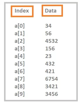
Data values are dummy values, you can understand after seeing the output, indexing starts from “0”.

Multidimensional Arrays

a 2D array can be defined as an array of arrays. The 2D array is organized as matrices which can be represented as the collection of rows and columns.

However, 2D arrays are created to implement a relational database look alike data structure. It provides ease of holding bulk data at once which can be passed to any number of functions wherever required.

How to declare 2D Array

The syntax of declaring a two dimensional array is very much similar to that of a one dimensional array, given as follows.

Int arr[max_rows][max_columns];  

However, it produces the data structure which looks like the following.

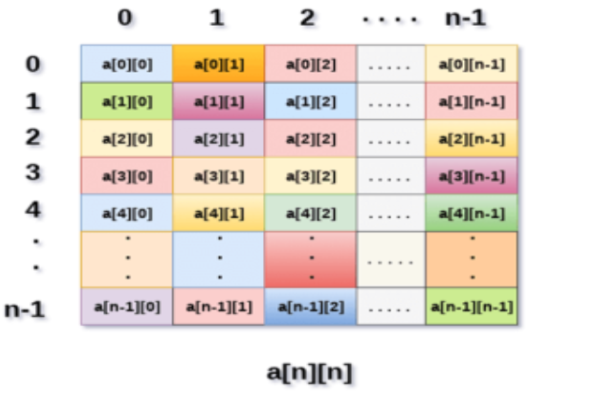
Fig 5:  Example

Above image shows the two-dimensional array, the elements are organized in the form of rows and columns. First element of the first row is represented by a [0][0] where the number shown in the first index is the number of that row while the number shown in the second index is the number of the column.

How do we access data in a 2D array?

Due to the fact that the elements of 2D arrays can be random accessed. Similar to one dimensional array, we can access the individual cells in a 2D array by using the indices of the cells. There are two indices attached to a particular cell, one is its row number while the other is its column number.

However, we can store the value stored in any particular cell of a 2D array to some variable x by using the following syntax.

Where i and j is the row and column number of the cell respectively.

We can assign each cell of a 2D array to 0 by using the following code:

Initializing 2D Arrays

We know that, when we declare and initialize a one-dimensional array in C programming simultaneously, we don't need to specify the size of the array. However, this will not work with 2D arrays. We will have to define at least the second dimension of the array.

The syntax to declare and initialize the 2D array is given as follows.

The number of elements that can be present in a 2D array will always be equal to (number of rows * number of columns).

Example: Storing User's data into a 2D array and printing it.

C Example:

Java Example

C# Example

Mapping 2D array to 1D array

When it comes to map a 2-dimensional array, most of us might think that why this mapping is required. However, 2 D arrays exists from the user point of view. 2D arrays are created to implement a relational database table lookalike data structure, in computer memory, the storage technique for 2D array is similar to that of a one-dimensional array.

The size of a two-dimensional array is equal to the multiplication of number of rows and the number of columns present in the array. We do need to map two-dimensional array to the one-dimensional array in order to store them in the memory.

A 3 X 3 two-dimensional array is shown in the following image. However, this array needs to be mapped to a one-dimensional array in order to store it into the memory.

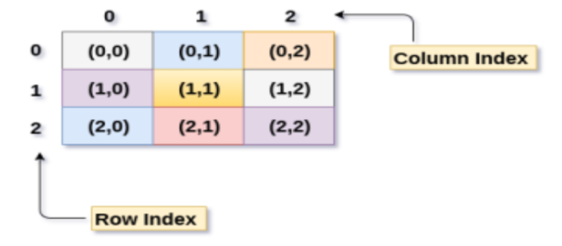
Fig 6: 3 X 3 two-dimensional array

There are two main techniques of storing 2D array elements into memory

1. Row Major ordering

In row major ordering, all the rows of the 2D array are stored into the memory contiguously. Considering the array shown in the above image, its memory allocation according to row major order is shown as follows.

First, the 1st row of the array is stored into the memory completely, then the 2nd row of the array is stored into the memory completely and so on till the last row.

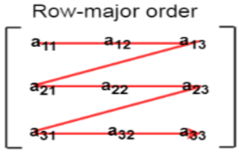
Fig 7: row major ordering

2. Column Major ordering

According to the column major ordering, all the columns of the 2D array are stored into the memory contiguously. The memory allocation of the array which is shown in in the above image is given as follows.

  First, the 1st column of the array is stored into the memory completely, then the 2nd row of the array is stored into the memory completely and so on till the last column of the array.

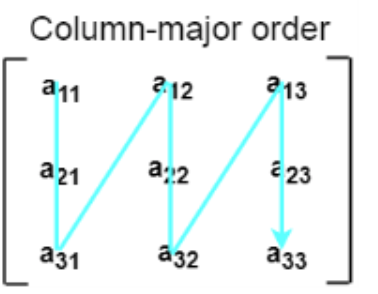
Fig 8: column major ordering

Calculating the Address of the random element of a 2D array

Due to the fact that there are two different techniques of storing the two-dimensional array into the memory, there are two different formulas to calculate the address of a random element of the 2D array.

By Row Major Order

If array is declared by a[m][n] where m is the number of rows while n is the number of columns, then address of an element a[i][j] of the array stored in row major order is calculated as,

Where, B. A. Is the base address or the address of the first element of the array a[0][0] .

Example:

By Column major order

If array is declared by a[m][n] where m is the number of rows while n is the number of columns, then address of an element a[i][j] of the array stored in row major order is calculated as,

Where BA is the base address of the array.

Example:

Key takeaway

1.12 Representation of Arrays: Row Major Order, and Column Major Order

Already Explain above.

1.13 Derivation of Index Formulae for 1-D,2-D,3-D and n-D Array

See above.

1.14 Application of arrays

●      Vectors and lists, which are fundamental parts of the C++ STL, are implemented using arrays.

●      Stacks and queues are also implemented using arrays.

●      Whenever possible, trees employ array implementation since arrays are easier to manage than pointers. Tress is then utilized to construct a variety of additional data structures.

●      Arrays are used to implement matrices, which are an important aspect of every computer language's mathematics library.

●      The graph's adjacency list is implemented using vectors, which are then implemented using arrays.

●      Binary search trees and balanced binary trees, which can be built using arrays, are used in data structures such as a heap, map, and set.

●      Multiple variables with the same name are stored in arrays.

●      Arrays are used to develop CPU scheduling algorithms.

●      Arrays are at the heart of all sorting algorithms.

1.15 Sparse Matrices and their representations

A matrix is a representation of certain rows and columns, to persist homogeneous data. It can also be called a double-dimensioned array.

Uses:

- To represent class hierarchy using Boolean square matrix

- For data encryption and decryption

- To represent traffic flow and plumbing in a network

- To implement graph theory of node representation

In this section we will see what is the sparse matrix and how we can represent them in memory. So a matrix will be a sparse matrix if most of the elements of it is 0. Another definition is, a matrix with a maximum of 1/3 non-zero elements (roughly 30% of m x n) is known as sparse matrix.

We use matrices in computers memory to do some operations in an efficient way. But if the matrices are sparse in nature, it may help us to do operations efficiently, but it will take up a larger space in memory. That space has no purpose. So, we will follow some other kind of structures to store sparse matrices.

Suppose we have a sparse matrix like below −

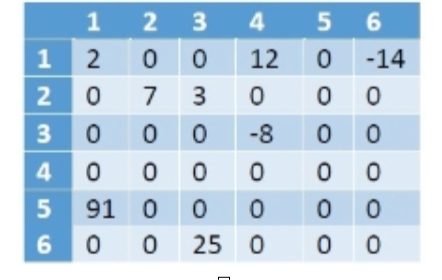
As we can see that there are 8 non-zero elements, and 28 zero-values. This matrix is taking 6*6 = 36 memory spaces. If the size of the matrix is larger, the wastage of space will be increased.

We can store the information about the sparse matrices using table structure. Suppose we will create a table called X like below −

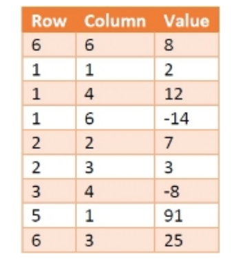
Here the first column is holding the Row number, and the second one is holding the column number. The third one is holding the data present at M[row, col]. Each row of this table is called triplets, as there are three parameters. The first triplet is holding the size information of the matrix. Row = 6 and Column = 6 is indicating that the matrix M is a 6 x 6 matrix. The value field is denoting the number of non-zero elements present in the array.

This table is also taking 9 * 3 = 36 amount of space, so where is the gain? Well, if the matrix size is 8*8 = 64, but only 8 elements are present, then also table X will take 36 units of space. We can see that there are fixed 3 columns, the number of rows varies with the number of non-zero elements. So, if there are T number of non-zero elements, then the space Complexity will be O(3*T) = O(T). For the matrix it will be O(m x n).

Key takeaway

Uses:

- To represent class hierarchy using Boolean square matrix

- For data encryption and decryption

- To represent traffic flow and plumbing in a network

- To implement graph theory of node representation

1.16 Linked lists: Array Implementation and Pointer Implementation of Singly Linked Lists, Doubly Linked List, Circularly Linked List

In programming, it is the most widely used linked list. When we talk about a linked list, we're talking about a singly linked list. The singly linked list is a data structure that is divided into two parts: the data portion and the address part, which contains the address of the next or successor node. A pointer is another name for the address component of a node.

Assume we have three nodes with addresses of 100, 200, and 300, respectively. The following diagram depicts the representation of three nodes as a linked list:

Fig 9: singly linked list

In the diagram above, we can see three separate nodes with addresses of 100, 200, and 300, respectively. The first node has the address of the next node, which is 200, the second has the address of the last node, which is 300, and the third has the NULL value in its address portion because it does not point to any node. A head pointer is a pointer that stores the address of the first node.

Because there is just one link in the linked list depicted in the figure, it is referred to as a singly linked list. Just forward traversal is permitted in this list; we can't go backwards because there is only one link in the list.

Representation of the node in a singly linked list

Struct node 

{ 

Int data; 

Struct node *next;

}

In the above diagram, we've constructed a user-made structure called a node, which has two members: one is data of integer type, and the other is the node type's pointer (next).

Doubly linked list

The doubly linked list, as its name implies, has two pointers. The doubly linked list can be described as a three-part linear data structure: the data component, the address part, and the other two address parts. A doubly linked list, in other terms, is a list with three parts in each node: one data portion, a pointer to the previous node, and a pointer to the next node.

Let's pretend we have three nodes with addresses of 100, 200, and 300, respectively. The representation of these nodes in a doubly-linked list is shown below:

Fig 10: doubly linked list

The node in a doubly-linked list contains two address portions, as shown in the diagram above; one part keeps the address of the next node, while the other half stores the address of the previous node. The address component of the first node in the doubly linked list is NULL, indicating that the prior node's address is NULL.

Representation of the node in a doubly linked list

Struct node 

{ 

Int data; 

Struct node *next; 

Struct node *prev;  

}  

In the above representation, we've constructed a user-defined structure called a node, which has three members: one is data of integer type, and the other two are pointers of the node type, i.e. next and prev. The address of the next node is stored in the next pointer variable, whereas the address of the previous node is stored in the prev pointer variable. The type of both the pointers, i.e., next and prev is struct node as both the pointers are storing the address of the node of the struct node type.

Circular linked list

A singly linked list is a type of circular linked list. The sole difference between a singly linked list and a circular linked list is that the last node in a singly linked list does not point to any other node, therefore its link portion is NULL. The circular linked list, on the other hand, is a list in which the last node connects to the first node, and the address of the first node is stored in the link section of the last node.

There are no nodes at the beginning or finish of the circular linked list. We can travel in either way, backwards or forwards. The following is a diagrammatic illustration of the circular linked list:

Struct node 

{ 

Int data; 

Struct node *next; 

} 

A circular linked list is a collection of elements in which each node is linked to the next and the last node is linked to the first. The circular linked list will be represented similarly to the singly linked list, as demonstrated below:

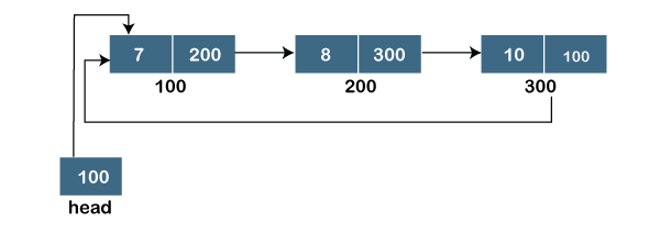
Fig 11: circular linked list

Key takeaway

1.17 Operations on a Linked List Insertion, Deletion, Traversal

Insertion

When placing a node into a linked list, there are three possible scenarios:

Insertion at the beginning

There's no need to look for the end of the list. If the list is empty, the new node becomes the list's head. Otherwise, we must connect the new node to the existing list's head and make the new node the list's head.

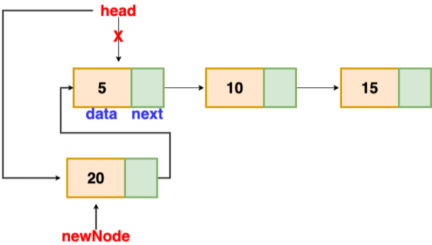
Fig 12: insertion at beginning

// function is returning the head of the singly linked-list

Node insertAtBegin(Node head, int val)

{

NewNode = new Node(val) // creating new node of linked list

If(head == NULL) // check if linked list is empty

Return newNode

Else // inserting the node at the beginning

{

NewNode.next = head

Return newNode

}

}

Insertion at the end

We'll go through the list till we reach the last node. The new node is then appended to the end of the list. It's worth noting that there are some exceptions, such as when the list is empty.

We will return the updated head of the linked list if the list is empty, because the inserted node is both the first and end node of the linked list in this case.

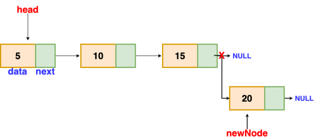
Fig 13: insertion at end

// the function is returning the head of the singly linked list

Node insertAtEnd(Node head, int val)

{

If( head == NULL ) // handing the special case

{

NewNode = new Node(val)

Head = newNode

Return head

}

Node temp = head

// traversing the list to get the last node

While( temp.next != NULL )

{

Temp = temp.next

}

NewNode = new Node(val)

Temp.next = newNode

Return head

}

Insertion after a given node

The reference to a node is passed to us, and the new node is put after it.

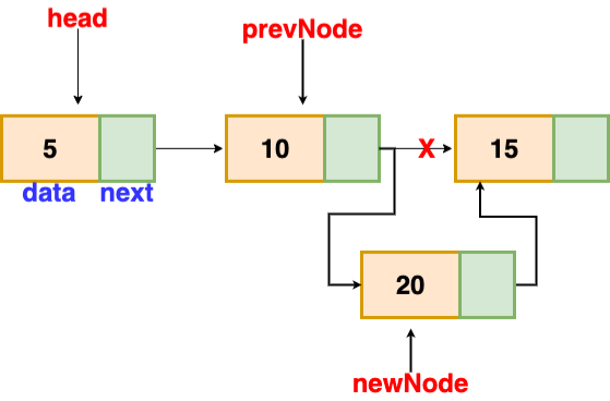
Fig 14: insertion after given node

Void insertAfter(Node prevNode, int val)

{

NewNode = new Node(val)

NewNode.next = prevNode.next

PrevNode.next = newNode

}

Deletion

These are the procedures to delete a node from a linked list.

There is a specific circumstance in which the first node is removed upon deletion. We must update the connected list's head in this case.

Fig 15: deleting a node in linked list

// this function will return the head of the linked list

Node deleteLL(Node head, Node del)

{

If(head == del) // if the node to be deleted is the head node

{

Return head.next // special case for the first Node

}

Node temp = head

While( temp.next != NULL )

{

If(temp.next == del) // finding the node to be deleted

{

Temp.next = temp.next.next

Delete del // free the memory of that Node

Return head

}

Temp = temp.next

}

Return head // if no node matches in the Linked List

}

Traversal

The goal is to work your way through the list from start to finish. We might want to print the list or search for a certain node in it, for example.

The traversal algorithm for a list

Void traverseLL(Node head) {

While(head != NULL)

{

Print(head.data)

Head = head.next

}

}

Key takeaway

1.18 Polynomial Representation and Addition Subtraction & Multiplications of Single variable & Two variables Polynomial

Polynomials can be represented in a number of different ways. These are the following:

●      By the use of arrays

●      By the use of Linked List

Representation of polynomial using Arrays

There may be times when you need to evaluate a large number of polynomial expressions and execute fundamental arithmetic operations on them, such as addition and subtraction. You'll need a mechanism to express the polynomials for this. The simplest method is to express a polynomial of degree 'n' and store the coefficient of the polynomial's n+1 terms in an array. As a result, each array element will have two values:

●      Coefficient and

●      Exponent

Polynomial of representation using linked lists

An ordered list of non-zero terms can be thought of as a polynomial. Each non-zero word is a two-tuple, containing two pieces of data:

●      The exponent part

●      The coefficient part

Multiplication

To multiply two polynomials, multiply the terms of one polynomial by the terms of the other polynomial. Assume the two polynomials have n and m terms respectively. A polynomial with n times m terms will be created as a result of this method.

For example, we can construct a linked list by multiplying  and

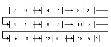
All of the terms we'll need to get the final outcome are in this linked list. The powers, on the other hand, do not sort it. It also has duplicate nodes with similar terms. We can merge sort the linked list depending on each node's power to get the final linked list:

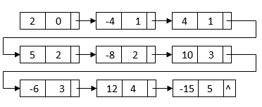
After sorting, the nodes with similar terms are clustered together. Then, for the final multiplication result, we can combine each set of like terms:

Code for Polynomial addition, subtraction and multiplication in C

#include<stdio.h>

#include<conio.h>

#include "poly.h"void main()

{

Clrscr();

Polynomial *p1,*p2,*sum,*sub,*mul;

Printf("\nENTER THE FIRST POLYNOMIAL.");

p1=createPolynomial();

Printf("\nENTER THE SECOND POLYNOMIAL.");

p2=createPolynomial();

Clrscr();

Printf("\nFIRST : ");

DisplayPolynomial(p1);

Printf("\nSECOND : ");

DisplayPolynomial(p2);

Printf("\n\nADDITION IS : ");

Sum=addPolynomial(p1,p2);

DisplayPolynomial(sum);

Printf("\n\nSUBTRACTION IS : ");

Sub=subPolynomial(p1, p2);

DisplayPolynomial(sub);

Printf("\n\nMULTIPLICATION IS : ");

Mul=mulPolynomial(p1, p2);

DisplayPolynomial(mul);

Getch();

}

Key takeaway

References: