Unit – 4
Graphs
Graph
A graph can be defined as group of vertices and edges that are used to connect these vertices. A graph can be seen as a cyclic tree, where the vertices (Nodes) maintain any complex relationship among them instead of having parent child relationship.
Definition
A graph G can be defined as an ordered set G (V, E) where V(G) represents the set of vertices and E(G) represents the set of edges which are used to connect these vertices.
A Graph G (V, E) with 5 vertices (A, B, C, D, E) and six edges ((A, B), (B, C), (C, E), (E, D), (D, B), (D, A)) is shown in the following figure.
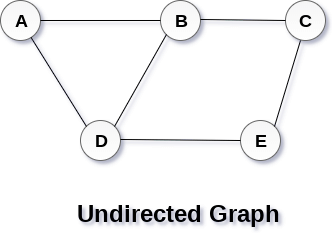
Fig 1– Undirected graph
Directed and Undirected Graph
A graph can be directed or undirected. However, in an undirected graph, edges are not associated with the directions with them. An undirected graph is shown in the above figure since its edges are not attached with any of the directions. If an edge exists between vertex A and B then the vertices can be traversed from B to A as well as A to B.
In a directed graph, edges form an ordered pair. Edges represent a specific path from some vertex A to another vertex B. Node A is called the initial node while node B is called terminal node.
A directed graph is shown in the following figure.
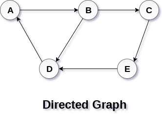
Fig 2– Directed graph
Graph Terminology
Path
A path can be defined as the sequence of nodes that are followed in order to reach some terminal node V from the initial node U.
Closed Path
A path will be called as closed path if the initial node is same as terminal node. A path will be closed path if V0=VN.
Simple Path
If all the nodes of the graph are distinct with an exception V0=VN, then such path P is called as closed simple path.
Cycle
A cycle can be defined as the path which has no repeated edges or vertices except the first and last vertices.
Connected Graph
A connected graph is the one in which some path exists between every two vertices (u, v) in V. There are no isolated nodes in connected graph.
Complete Graph
A complete graph is the one in which every node is connected with all other nodes. A complete graph contain n(n-1)/2 edges where n is the number of nodes in the graph.
Weighted Graph
In a weighted graph, each edge is assigned with some data such as length or weight. The weight of an edge e can be given as w(e) which must be a positive (+) value indicating the cost of traversing the edge.
Digraph
A digraph is a directed graph in which each edge of the graph is associated with some direction and the traversing can be done only in the specified direction.
Loop
An edge that is associated with the similar end points can be called as Loop.
Adjacent Nodes
If two nodes u and v are connected via an edge e, then the nodes u and v are called as neighbours or adjacent nodes.
Degree of the Node
A degree of a node is the number of edges that are connected with that node. A node with degree 0 is called as isolated node.
Key takeaway
- A graph can be defined as group of vertices and edges that are used to connect these vertices.
- A graph can be seen as a cyclic tree, where the vertices (Nodes) maintain any complex relationship among them instead of having parent child relationship.
Graph Representation
By Graph representation, we simply mean the technique which is to be used in order to store some graph into the computer's memory.
There are two ways to store Graph into the computer's memory.
1. Sequential Representation
In sequential representation, we use an adjacency matrix to store the mapping represented by vertices and edges. In adjacency matrix, the rows and columns are represented by the graph vertices. A graph having n vertices, will have a dimension n x n.
An entry Mij in the adjacency matrix representation of an undirected graph G will be 1 if there exists an edge between Vi and Vj.
An undirected graph and its adjacency matrix representation is shown in the following figure.

Fig 3– Undirected graph and its adjacency matrix
In the above figure, we can see the mapping among the vertices (A, B, C, D, E) is represented by using the adjacency matrix which is also shown in the figure.
There exists different adjacency matrices for the directed and undirected graph. In directed graph, an entry Aij will be 1 only when there is an edge directed from Vi to Vj.
A directed graph and its adjacency matrix representation is shown in the following figure.
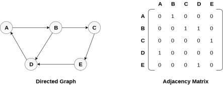
Fig 4- Directed graph and its adjacency matrix
Representation of weighted directed graph is different. Instead of filling the entry by 1, the Non- zero entries of the adjacency matrix are represented by the weight of respective edges.
The weighted directed graph along with the adjacency matrix representation is shown in the following figure.
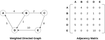
Fig 5 - Weighted directed graph
Key takeaway
- By Graph representation, we simply mean the technique which is to be used in order to store some graph into the computer's memory.
- There are two ways to store Graph into the computer's memory.
Linked Representation
In the linked representation, an adjacency list is used to store the Graph into the computer's memory.
Consider the undirected graph shown in the following figure and check the adjacency list representation.

Fig 6- Undirected graph in adjacency list
An adjacency list is maintained for each node present in the graph which stores the node value and a pointer to the next adjacent node to the respective node. If all the adjacent nodes are traversed then store the NULL in the pointer field of the last node of the list. The sum of the lengths of adjacency lists is equal to twice of the number of edges present in an undirected graph.
Consider the directed graph shown in the following figure and check the adjacency list representation of the graph.
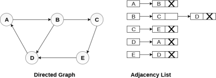
Fig 7- Directed graph in adjacency list
In a directed graph, the sum of lengths of all the adjacency lists is equal to the number of edges present in the graph.
In the case of weighted directed graph, each node contains an extra field that is called the weight of the node. The adjacency list representation of a directed graph is shown in the following figure.

Fig 8- weighted directed graph
Key takeaway
- In the linked representation, an adjacency list is used to store the Graph into the computer's memory.
- An adjacency list is maintained for each node present in the graph which stores the node value and a pointer to the next adjacent node to the respective node.
We use an adjacency matrix to store the mapping represented by vertices and edges. In the adjacency matrix, the rows and columns are represented by the graph vertices. A graph having n vertices, will have a dimension n x n.
In the linked representation, an adjacency list is used to store the Graph into the computer's memory.
Depth First Search is an algorithm for traversing or searching a graph.
It starts from some node as the root node and explores each and every branch of that node before backtracking to the parent node.
DFS is an uninformed search that progresses by expanding the first child node of the graph that appears and thus going deeper and deeper until a goal node is found, or until it hits a node that has no children.
Then the search backtracks, returning to the most recent node it hadn't finished exploring. In a non-recursive implementation, all freshly expanded nodes are added to a LIFO stack for expansion.
Steps for implementing Depth first search
Step 1: - Define an array A or Vertex that store Boolean values, its size should be greater or equal to the number of vertices in the graph G.
Step 2: - Initialize the array A to false
Step 3: - For all vertices v in G
If A[v] = false
Process (v)
Step 4: - Exit
Algorithm for DFS
DFS(G)
{
For each v in V, //for loop V+1 times
{
Color[v]=white; // V times
p[v]=NULL; // V times
}
Time=0; // constant time O (1)
For each u in V, //for loop V+1 times
If (color[u]==white) // V times
DFSVISIT(u) // call to DFSVISIT(v), at most V times O(V)
}
DFSVISIT(u)
{
Color[u]=gray; // constant time
t[u] = ++time;
For each v in Adj(u) // for loop
If (color[v] == white)
{
p[v] = u;
DFSVISIT(v); // call to DFSVISIT(v)
}
Color[u] = black; // constant time
f[u]=++time; // constant time
}
DFS algorithm used to solve following problems:
● Testing whether graph is connected.
● Computing a spanning forest of graph.
● Computing a path between two vertices of graph or equivalently reporting that no such path exists.
● Computing a cycle in graph or equivalently reporting that no such cycle exists.
Analysis of DFS
In the above algorithm, there is only one DFSVISIT(u) call for each vertex u in the vertex set V. Initialization complexity in DFS(G) for loop is O(V). In second for loop of DFS(G), complexity is O(V) if we leave the call of DFSVISIT(u).
Now, let us find the complexity of function DFSVISIT(u)
The complexity of for loop will be O(deg(u)+1) if we do not consider the recursive call to DFSVISIT(v). For recursive call to DFSVISIT(v), (complexity will be O(E) as
Recursive call to DFSVISIT(v) will be at most the sum of degree of adjacency for all vertex v in the vertex set V. It can be written as ∑ |Adj(v)|=O(E) vεV
The running time of DSF is (V + E).
Breadth First Search
It is an uninformed search methodology which first expand and examine all nodes of graph systematically in search of the solution in the sequence and then go at the deeper level. In other words, it exhaustively searches the entire graph without considering the goal until it finds it.
From the standpoint of the algorithm, all child nodes obtained by expanding a node are added to a FIFO queue. In typical implementations, nodes that have not yet been examined for their neighbors are placed in some container (such as a queue or linked list) called "open" and then once examined are placed in the container "closed".
Steps for implementing Breadth first search
Step 1: - Initialize all the vertices by setting Flag = 1
Step 2: - Put the starting vertex A in Q and change its status to the waiting state by setting Flag = 0
Step 3: - Repeat through step 5 while Q is not NULL
Step 4: - Remove the front vertex v of Q. Process v and set the status of v to the processed status by setting Flag = -1
Step 5: - Add to the rear of Q all the neighbour of v that are in the ready state by setting Flag = 1 and change their status to the waiting state by setting flag = 0
Step 6: - Exit
Algorithm for BFS
BFS (G, s)
{
For each v in V - {s} // for loop {
Color[v]=white;
d[v]= INFINITY;
p[v]=NULL;
}
Color[s] = gray;
d[s]=0;
p[s]=NULL;
Q = ø; // Initialize queue is empty
Enqueue(Q, s); /* Insert start vertex s in Queue Q */
While Q is nonempty // while loop
{
u = Dequeue[Q]; /* Remove an element from Queue Q*/
For each v in Adj[u] // for loop
{ if (color[v] == white) /*if v is unvisted*/
{
Color[v] = gray; /* v is visted */
d[v] = d[u] + 1; /*Set distance of v to no. Of edges from s to u*/
p[v] = u; /*Set parent of v*/
Enqueue(Q,v); /*Insert v in Queue Q*/
}
}
Color[u] = black; /*finally visted or explored vertex u*/
}
}
Breadth First Search algorithm used in
● Prim's MST algorithm.
● Dijkstra's single source shortest path algorithm.
● Testing whether graph is connected.
● Computing a cycle in graph or reporting that no such cycle exists.
Analysis of BFS
In this algorithm first for loop executes at most O(V) times.
While loop executes at most O(V) times as every vertex v in V is enqueued only once in the Queue Q. Every vertex is enqueued once and dequeued once so queuing will take at most O(V) time.
Inside while loop, there is for loop which will execute at most O(E) times as it will be at most the sum of degree of adjacency for all vertex v in the vertex set V.
Which can be written as
∑ |Adj(v)|=O(E)
vεV
Total running time of BFS is O(V + E).
Like depth first search, BFS traverse a connected component of a given graph and defines a spanning tree.
Space complexity of DFS is much lower than BFS (breadth-first search). It also lends itself much better to heuristic methods of choosing a likely-looking branch. Time complexity of both algorithms are proportional to the number of vertices plus the number of edges in the graphs they traverse.
Key takeaways
- Depth First Search is an algorithm for traversing or searching a graph.
- DFS is an uninformed search that progresses by expanding the first child node of the graph that appears and thus going deeper and deeper until a goal node is found, or until it hits a node that has no children.
- BFS is an uninformed search methodology which first expand and examine all nodes of graph systematically in search of the solution in the sequence and then goes to the deeper level.
- In other words, it exhaustively searches the entire graph without considering the goal until it finds it.
Given an undirected graph, print all connected components line by line. For example consider the following graph.
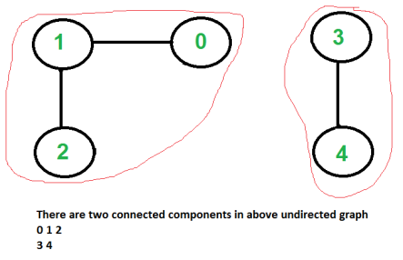
We strongly recommend to minimize your browser and try this yourself first.
We have discussed algorithms for finding strongly connected components in directed graphs in the following posts.
Kosaraju’s algorithm for strongly connected components.
Tarjan’s Algorithm to find Strongly Connected Components
Finding connected components for an undirected graph is an easier task. We simple need to do either BFS or DFS starting from every unvisited vertex, and we get all strongly connected components. Below are steps based on DFS.
1) Initialize all vertices as not visited.
2) Do the following for every vertex 'v'.
(a) If 'v' is not visited before, call DFSUtil(v)
(b) Print new line character
DFSUtil(v)
1) Mark 'v' as visited.
2) Print 'v'
3) Do the following for every adjacent 'u' of 'v'.
If 'u' is not visited, then recursively call DFSUtil(u)
Below is the implementation of the above algorithm.
// C++ program to print connected components in
// an undirected graph
#include <iostream>
#include <list>
Using namespace std;
// Graph class represents a undirected graph
// using adjacency list representation
Class Graph {
Int V; // No. Of vertices
// Pointer to an array containing adjacency lists
List<int>* adj;
// A function used by DFS
Void DFSUtil(int v, bool visited[]);
Public:
Graph(int V); // Constructor
~Graph();
Void addEdge(int v, int w);
Void connectedComponents();
};
// Method to print connected components in an
// undirected graph
Void Graph::connectedComponents()
{
// Mark all the vertices as not visited
Bool* visited = new bool[V];
For (int v = 0; v < V; v++)
Visited[v] = false;
For (int v = 0; v < V; v++) {
If (visited[v] == false) {
// print all reachable vertices
// from v
DFSUtil(v, visited);
Cout << "\n";
}
}
Delete[] visited;
}
Void Graph::DFSUtil(int v, bool visited[])
{
// Mark the current node as visited and print it
Visited[v] = true;
Cout << v << " ";
// Recur for all the vertices
// adjacent to this vertex
List<int>::iterator i;
For (i = adj[v].begin(); i != adj[v].end(); ++i)
If (!visited[*i])
DFSUtil(*i, visited);
}
Graph::Graph(int V)
{
This->V = V;
Adj = new list<int>[V];
}
Graph::~Graph() { delete[] adj; }
// method to add an undirected edge
Void Graph::addEdge(int v, int w)
{
Adj[v].push_back(w);
Adj[w].push_back(v);
}
// Driver code
Int main()
{
// Create a graph given in the above diagram
Graph g(5); // 5 vertices numbered from 0 to 4
g.addEdge(1, 0);
g.addEdge(2, 3);
g.addEdge(3, 4);
Cout << "Following are connected components \n";
g.connectedComponents();
Return 0;
}
Output:
0 1
2 3 4
Time complexity of the above solution is O (V + E) as it does simple DFS for a given graph.
Key takeaway
- Finding connected components for an undirected graph is an easier task.
- We simple need to do either BFS or DFS starting from every unvisited vertex, and we get all strongly connected components. Below are steps based on DFS.
1) Initialize all vertices as not visited.
2) Do the following for every vertex 'v'.
(a) If 'v' is not visited before, call DFSUtil(v)
(b) Print new line character
A spanning tree is a subset of Graph G that covers all of the vertices with the fewest amount of edges feasible. As a result, a spanning tree has no cycles and cannot be disconnected.
We can deduce from this definition that every linked and undirected Graph G contains at least one spanning tree. Because a disconnected graph cannot be spanned to all of its vertices, it lacks a spanning tree.
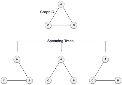
Fig 9: Spanning tree
From a single full graph, we discovered three spanning trees. The greatest number of spanning trees in a full undirected graph is nn-2, where n is the number of nodes. Because n is 3 in the example above, 33-2 = 3 spanning trees are conceivable.
Properties of spanning tree
We now know that a graph can contain many spanning trees. A few features of the spanning tree related to graph G are listed below.
● There can be more than one spanning tree in a linked graph G.
● The number of edges and vertices in all conceivable spanning trees of graph G is the same.
● There is no cycle in the spanning tree (loops).
● When one edge is removed from the spanning tree, the graph becomes unconnected, i.e. the spanning tree becomes minimally connected.
● When one edge is added to the spanning tree, a circuit or loop is created, indicating that the spanning tree is maximally acyclic.
Application of spanning tree
The spanning tree is used to discover the shortest path between all nodes in a graph. The use of spanning trees is common in a variety of situations.
● Civil Network Planning
● Computer Network Routing Protocol
● Cluster Analysis
Let's look at an example to help us comprehend. Consider the city network as a large graph, and the current objective is to deploy telephone lines in such a way that we can link to all city nodes with the bare minimum of lines. The spanning tree enters the scene at this point.
Key takeaway
- A spanning tree is a subset of Graph G that covers all of the vertices with the fewest amount of edges feasible.
- As a result, a spanning tree has no cycles and cannot be disconnected.
In the Greedy approach MST (Minimum Spanning Trees) is used to find the cost or the minimum path. Let G= (V, E) be an undirected connected graph, also T= (V’, E’) be a subgraph of the spanning tree G if and only if T is a tree.
Spanning trees are usually used to get an independent set of circuit’s equations in the electrical network. Once the spanning tree is obtained, suppose B is a set of edges not present in the spanning tree then adding one edge from B will form an electrical cycle.
A spanning tree is a minimal subgraph G’ of G such that V (G’) =V (G) and G’ is connected by a minimal subgraph. Any connected graph with n vertices must have at least n-1 edges and all connected graphs with n-1 edges are trees. The spanning trees of G will represent all feasible choices. The best spanning tree is tree with the minimum cost.
The cost of the spanning tree is nothing but the sum of the cost of the edges in that tree. Any tree consisting of edges of a graph and including all the vertices of the graph is known as a “Spanning Tree”.
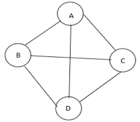
Fig 10: Graph with vertices
The above figure shows a graph with four vertices and some of its spanning tree are shown as below:

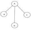

Fig 11: Spanning tree
Minimum Cost Spanning Tree
Definition: Let G= (V, E) be an undirected connected graph. A sub-graph t= (V, E’) of G is a spanning tree of G if t is a tree.
Spanning trees have many applications. It can be used to obtain an independent set of circuit equations for an electric network.
In Greedy approach a Minimum Cost Spanning Tree is created using the given graph G. Let us consider a connected weighted graph G our aim here is to create a spanning tree T for G such that the sum of the weights of the tree edges in T is as small as possible.
To do so the greedy approach is to draw the tree by selecting edge by edge. Initially the first edge is selected and then the next edge is selected by considering the lowest cost. The process selecting edges one by one goes on till all the vertices have been visited with the edges of the minimum cost.
There are two ways to do so: -
- Kruskal’s Algorithm: - Here edges of the graph are considered in non-decreasing order of cost. The set of T of edges so far selected for the spanning tree should be such that it is possible to complete T into a tree.
2. Prim’s Algorithm: - Here the set of edges so far selected should from a tree. Now if A is the set of edges selected so far, then A has to form a tree. The next edge (u, v) to be included in A is a minimum cost edge not in A with the property that A ∪ {(u, v)} also results in a tree.
Key takeaway
- In the Greedy approach Minimum Spanning Trees is used to find the cost or the minimum path.
- Spanning trees have many applications. It can be used to obtain an independent set of circuit equations for an electric network.
- A spanning tree is a minimal subgraph G’ of G such that V (G’) =V (G) and G’ is connected by a minimal subgraph.
Prim’s algorithm
● If A is the set of edges selected so far, then A forms a tree.
● The next edge (u, v) to be included in A is a minimum cost edge not in A with the property that A U {u, v} is also a tree.
● Steps to solve the prim's algorithm:
Step 1: remove all loops and parallel edges
Step 2: chose any arbitrary node as root node
Step 3: check the outgoing edges and chose edge with the less value
Step 4: find the optimal solution by adding all the minimum cost of edges.
● Example :
To find the MST, apply Prim's algorithm to the following graph.
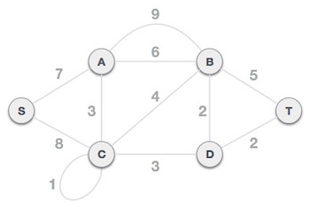
Solution:
Step1: Remove all loops and parallel edges
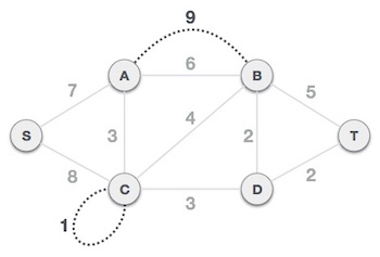
From the provided graph, remove any loops and parallel edges. If there are parallel edges, keep the one with the lowest cost and discard the others.
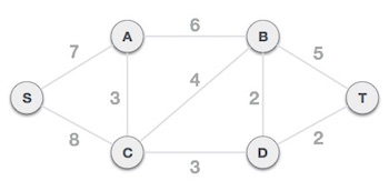
Step 2: Choose any arbitrary node as root node
In this scenario, the root node of Prim's spanning tree is S node. Because this node is picked at random, any node can be the root node. It's understandable to wonder why any video can be a root node. So, all the nodes of a graph are included in the spanning tree, and because it is connected, there must be at least one edge that connects it to the rest of the tree.
Step 3: Check outgoing edges and select the one with less cost
We can see that S, A and S, C are two edges with weights of 7 and 8, respectively, after selecting the root node S. The edge S, A is chosen since it is smaller than the other.
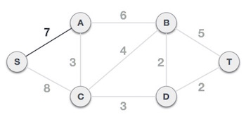
The tree S-7-A is now viewed as a single node, and all edges emanating from it are checked. We choose the one with the lowest price and put it on the tree.

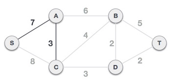
The S-7-A-3-C tree is generated after this phase. Now we'll treat it like a node again, and we'll double-check all of the edges. However, we will only select the lowest-cost advantage. In this scenario, the new edge is C-3-D, which costs less than the other edges' costs of 8, 6, 4, and so on.
Following the addition of node D to the spanning tree, we now have two edges with the same cost, namely D-2-T and D-2-B. As a result, we can use any one. However, at the next step, edge 2 will again be the least expensive. As a result, we've drawn a spanning tree that includes both edges.
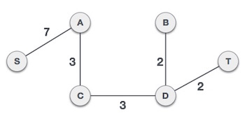
It's possible that the output spanning tree of two distinct algorithms for the same graph is the same.
Algorithm Prim (E, cost, n, t)
//E is the set of edges in G cost (1: n,1: n) is the adjacency matrix such at cost (i, j) is a +ve //real number or cost (i, j) is ∞ if no edge (i, j) exists. A minimum cost spanning tree is //computed and stored as a set of edges in the array T (1: n-1,1:2). (T(i,1), T(i,2) is an edge //in minimum cost spanning tree. The final cost is returned.
{
Let (k,l) to be an edge of minimum cost in E;
Mincost ß cost (k,l);
(T(1,1) T(1,2) )ß (k,l);
For iß 1 to n do // initialing near
If cost (i,L) < cost (I,k) then near (i) ß L ;
Else near (i) ß k;
Near(k) ß near (l) ß 0;
For i ß 2 to n-1 do
{
//find n-2 additional edges for T
Let j be an index such that near (J) ¹ 0 and
Cost (J, near(J)) is minimum;
(T(i, 1), T(i, 2)) ß (j, NEAR (j));
Mincost ß mincost + cost (j, near (j));
Near (j) ß 0;
For k ß 1 to n do // update near[]
If near (k) ¹ 0 and cost(k near (k)) > cost(k,j) then NEAR (k) ß j;
}
Return mincost;
}
Complexities:
A simple implementation using an adjacency matrix graph representation and searching an array of weights to find the minimum weight edge to add requires O(V2) running time.
Using a simple binary heap data structure and an adjacency list representation, Prim's algorithm can be shown to run in time O(E log V) where E is the number of edges and V is the number of vertices.
Using a more sophisticated Fibonacci heap, this can be brought down to O(E + V log V), which is asymptotically faster when the graph is dense enough that E is Ω(V).
Kruskal algorithm
Kruskal's Algorithm assembles the spanning tree by adding edges individually into a developing crossing tree. Kruskal's calculation follows a greedy approach as in every cycle it finds an edge which has least weight and add it to the developing traversing tree.
Calculation Steps:
Sort the chart edges concerning their loads.
Begin adding edges to the MST from the edge with the littlest load until the edge of the biggest weight.
Just add edges which doesn't frame a cycle, edges which interface just separated parts.
So now the inquiry is the means by which to check if vertices are associated or not?
This could be done using DFS which starts from the first vertex, then check if the second vertex is visited or not. But DFS will make time complexity large as it has an order of O(V+E) where V is the number of vertices, E is the number of edges. So the best solution is "Disjoint Sets":
Disjoint sets will be setting whose crossing point is the unfilled set so it implies that they don't share any component practically speaking.
Think about after model:
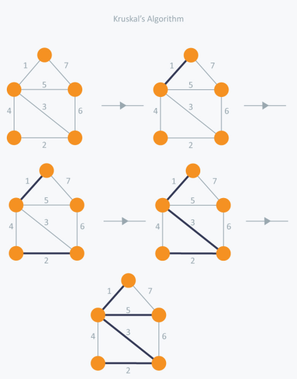
In Kruskal's algorithm, we pick the edge with the lowest weight for each iteration. So, first of all, we will start with the lowest weighted edge, i.e. the edges with weight 1. We would choose the second lowest weighted edge after that, i.e. the edge with weight 2. Notice that these two edges are absolutely disjointed. The third lowest weighted edge will now be the next edge, i.e. the edge with weight 3, which connects the two disjoint parts of the graph. Still, with weight 4, we are not able to choose the edge that will create a loop and we can't get any cycles. But we are going to pick the fifth lowest weighted edge, i.e. the 5th weighted edge. Now the other two sides are trying to build loops, so we're going to forget them. In the end, we end up with a minimum spanning tree with total cost 11 (= 1 + 2 + 3 + 5).
Time Complexity:
In Kruskal’s algorithm, the most time-consuming operation is sorting because the total complexity of the Disjoint-Set operations will be O(ElogV), which is the overall Time Complexity of the algorithm.
Key takeaway
- Prim's algorithm is a vertex algorithm based on
- Prim's algorithm-needs priority queue for the nearest vertex position.\
- Kruskal's Algorithm assembles the spanning tree by adding edges individually into a developing crossing tree.
- Kruskal's calculation follows a greedy approach as in every cycle it finds an edge which has least weight and add it to the developing traversing tree.
Transitive Closure is the reachability matrix to reach from vertex u to vertex v of a graph. One graph is given, we have to find a vertex v which is reachable from another vertex u, for all vertex pairs (u, v).
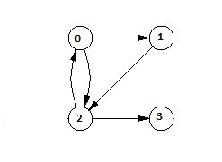
Fig 12- Transitive Closure
The final matrix is the Boolean type. When there is a value 1 for vertex u to vertex v, it means that there is at least one path from u to v.
Input and Output
Input:
1 1 0 1
0 1 1 0
0 0 1 1
0 0 0 1
Output:
The matrix of transitive closure
1 1 1 1
0 1 1 1
0 0 1 1
0 0 0 1
Algorithm
TransClosure(graph)
Input: The given graph.
Output: Transitive Closure matrix.
Begin
Copy the adjacency matrix into another matrix named transMat
For any vertex k in the graph, do
For each vertex i in the graph, do
For each vertex j in the graph, do
TransMat[i, j] := transMat[i, j] OR (transMat[i, k]) AND transMat[k, j])
Done
Done
Done
Display the transMat
End
<2>Example
#include<iostream>
#include<vector>
#define NODE 4
Using namespace std;
/* int graph[NODE][NODE] = {
{0, 1, 1, 0},
{0, 0, 1, 0},
{1, 0, 0, 1},
{0, 0, 0, 0}
}; */
Int graph[NODE][NODE] = {
{1, 1, 0, 1},
{0, 1, 1, 0},
{0, 0, 1, 1},
{0, 0, 0, 1}
};
Int result[NODE][NODE];
Void transClosure() {
For(int i = 0; i<NODE; i++)
For(int j = 0; j<NODE; j++)
Result[i][j] = graph[i][j]; //initially copy the graph to the result matrix
For(int k = 0; k<NODE; k++)
For(int i = 0; i<NODE; i++)
For(int j = 0; j<NODE; j++)
Result[i][j] = result[i][j] || (result[i][k] && result[k][j]);
For(int i = 0; i<NODE; i++) { //print the result matrix
For(int j = 0; j<NODE; j++)
Cout << result[i][j] << " ";
Cout << endl;
}
}
Int main() {
TransClosure();
}
Output
1 1 1 1
0 1 1 1
0 0 1 1
0 0 0 1
Key takeaway
- Transitive Closure it the reachability matrix to reach from vertex u to vertex v of a graph.
- One graph is given, we have to find a vertex v which is reachable from another vertex u, for all vertex pairs (u, v).

3. The final matrix is the Boolean type. When there is a value 1 for vertex u to vertex v, it means that there is at least one path from u to v.
Floyd-Warshall Algorithm
Let the vertices of G be V = {1, 2........n} and consider a subset {1, 2........k} of vertices for some k. For any pair of vertices i, j ∈ V, considered all paths from i to j whose intermediate vertices are all drawn from {1, 2.......k}, and let p be a minimum weight path from amongst them. The Floyd-Warshall algorithm exploits a link between path p and shortest paths from i to j with all intermediate vertices in the set {1, 2.......k-1}. The link depends on whether or not k is an intermediate vertex of path p.
If k is not an intermediate vertex of path p, then all intermediate vertices of path p are in the set {1, 2........k-1}. Thus, the shortest path from vertex i to vertex j with all intermediate vertices in the set {1, 2.......k-1} is also the shortest path i to j with all intermediate vertices in the set {1, 2.......k}.
If k is an intermediate vertex of path p, then we break p down into i → k → j.
Let dij(k) be the weight of the shortest path from vertex i to vertex j with all intermediate vertices in the set {1, 2.......k}.
A recursive definition is given by

FLOYD - WARSHALL (W)
1. n ← rows [W].
2. D0 ← W
3. For k ← 1 to n
4. Do for i ← 1 to n
5. Do for j ← 1 to n
6. Do dij(k) ← min (dij(k-1),dik(k-1)+dkj(k-1) )
7. Return D(n)
The strategy adopted by the Floyd-Warshall algorithm is Dynamic Programming. The running time of the Floyd-Warshall algorithm is determined by the triply nested for loops of lines 3-6. Each execution of line 6 takes O (1) time. The algorithm thus runs in time θ(n3 ).
Example: Apply Floyd-Warshall algorithm for constructing the shortest path. Show that matrices D(k) and π(k) computed by the Floyd-Warshall algorithm for the graph.
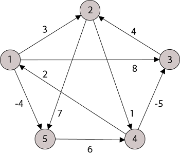
Solution:


Step (i) When k = 0
 | 3 | 8 | ∞ | -4 |  | 1 | 1 | Nil | 1 |
∞ | 0 | ∞ | 1 | 7 | Nil | Nil | Nil | 2 | 2 |
∞ | 4 | 0 | -5 | ∞ | Nil | 3 | Nil | 3 | Nil |
2 | ∞ | ∞ | 0 | ∞ | 4 | Nil | Nil | Nil | Nil |
∞ | ∞ | ∞ | 6 | 0 | Nil | Nil | Nil | 5 | Nil |
Step (ii) When k =1


 | 3 | 8 | ∞ | -4 |  | 1 | 1 | Nil | 1 |
∞ | 0 | ∞ | 1 | 7 | Nil | Nil | Nil | 2 | 2 |
∞ | 4 | 0 | -5 | ∞ | Nil | 3 | Nil | 3 | Nil |
2 | 5 | 10 | 0 | -2 | 4 | 1 | 1 | Nil | 1 |
∞ | ∞ | ∞ | 6 | 0 | Nil | Nil | Nil | 5 | Nil |
Step (iii) When k = 2


Step (iv) When k = 3
 | 0 | 3 | 8 | -4 |  | 1 | 1 | 3 | 1 |
∞ | 0 | ∞ | 1 | 7 | Nil | Nil | Nil | 2 | 2 |
∞ | 4 | 0 | -5 | 11 | Nil | 3 | Nil | 3 | 2 |
2 | 5 | 10 | 0 | -2 | 4 | 1 | 1 | Nil | 1 |
∞ | ∞ | ∞ | 6 | 0 | Nil | Nil | Nil | 5 | Nil |
Step (v) When k = 4


 | 3 | 8 | 3 | -4 |  | 1 | 1 | 3 | 1 |
3 | 0 | 11 | 1 | -1 | 4 | Nil | 4 | 2 | 2 |
-3 | 0 | 0 | -5 | -7 | 4 | 4 | NIL | 3 | 4 |
2 | 5 | 10 | 0 | -2 | 4 | 1 | 1 | NIL | 1 |
8 | 11 | 16 | 6 | 0 | 4 | 4 | 4 | 5 | NIL |
Step (vi) When k = 5


 | 3 | 8 | 3 | -4 |  | 1 | 1 | 5 | 1 |
3 | 0 | 11 | 1 | -1 | 4 | Nil | 4 | 2 | 4 |
-3 | 0 | 0 | -5 | -7 | 4 | 4 | Nil | 3 | 4 |
2 | 5 | 10 | 0 | -2 | 4 | 1 | 1 | NIL | 1 |
8 | 11 | 16 | 6 | 0 | 4 | 4 | 4 | 5 | NIL |
TRANSITIVE- CLOSURE (G)
1. n ← |V[G]|
2. For i ← 1 to n
3. Do for j ← 1 to n
4. Do if i = j or (i, j) ∈ E [G]
5. The ← 1
6. Else ← 0
7. For k ← 1 to n
8. Do for i ← 1 to n
9. Do for j ← 1 to n
10. Dod ij(k) ←
11. Return T(n).
Dijkstra's Algorithm
It is a greedy algorithm that solves the single-source shortest path problem for a directed graph G = (V, E) with nonnegative edge weights, i.e., w (u, v) ≥ 0 for each edge (u, v) ∈ E.
Dijkstra's Algorithm maintains a set S of vertices whose final shortest - path weights from the source s have already been determined. That's for all vertices v ∈ S; we have d [v] = δ (s, v). The algorithm repeatedly selects the vertex u ∈ V - S with the minimum shortest - path estimate, insert u into S and relaxes all edges leaving u.
Because it always chooses the "lightest" or "closest" vertex in V - S to insert into set S, it is called as the greedy strategy.
Dijkstra's Algorithm (G, w, s)
1. INITIALIZE - SINGLE - SOURCE (G, s)
2. S←∅
3. Q←V [G]
4. While Q ≠ ∅
5. Do u ← EXTRACT - MIN (Q)
6. S ← S ∪ {u}
7. For each vertex v ∈ Adj [u]
8. Do RELAX (u, v, w)
Analysis: The running time of Dijkstra's algorithm on a graph with edges E and vertices V can be expressed as a function of |E| and |V| using the Big - O notation. The simplest implementation of the Dijkstra's algorithm stores vertices of set Q in an ordinary linked list or array, and operation Extract - Min (Q) is simply a linear search through all vertices in Q. In this case, the running time is O (|V2 |+|E|=O(V2 ).
Example:

Solution:
Step1: Q =[s, t, x, y, z]
We scanned vertices one by one and find out its adjacent. Calculate the distance of each adjacent to the source vertices.
We make a stack, which contains those vertices which are selected after computation of shortest distance.
Firstly we take's' in stack M (which is a source)
- M = [S] Q = [t, x, y, z]
Step 2: Now find the adjacent of s that are t and y.
- Adj [s] → t, y [Here s is u and t and y are v]
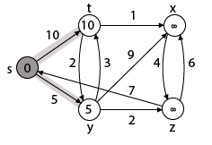
Case - (i) s → t
d [v] > d [u] + w [u, v]
d [t] > d [s] + w [s, t]
∞ > 0 + 10 [false condition]
Then d [t] ← 10
π [t] ← 5
Adj [s] ← t, y
Case - (ii) s→ y
d [v] > d [u] + w [u, v]
d [y] > d [s] + w [s, y]
∞ > 0 + 5 [false condition]
∞ > 5
Then d [y] ← 5
π [y] ← 5
By comparing case (i) and case (ii)
Adj [s] → t = 10, y = 5
y is shortest
y is assigned in 5 = [s, y]
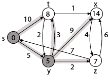
Step 3: Now find the adjacent of y that is t, x, z.
- Adj [y] → t, x, z [Here y is u and t, x, z are v]
Case - (i) y →t
d [v] > d [u] + w [u, v]
d [t] > d [y] + w [y, t]
10 > 5 + 3
10 > 8
Then d [t] ← 8
π [t] ← y
Case - (ii) y → x
d [v] > d [u] + w [u, v]
d [x] > d [y] + w [y, x]
∞ > 5 + 9
∞ > 14
Then d [x] ← 14
π [x] ← 14
Case - (iii) y → z
d [v] > d [u] + w [u, v]
d [z] > d [y] + w [y, z]
∞ > 5 + 2
∞ > 7
Then d [z] ← 7
π [z] ← y
By comparing case (i), case (ii) and case (iii)
Adj [y] → x = 14, t = 8, z =7
z is shortest
z is assigned in 7 = [s, z]
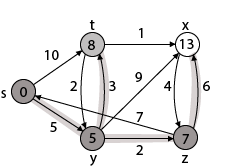
Step - 4 Now we will find adj [z] that are s, x
- Adj [z] → [x, s] [Here z is u and s and x are v]
Case - (i) z → x
d [v] > d [u] + w [u, v]
d [x] > d [z] + w [z, x]
14 > 7 + 6
14 > 13
Then d [x] ← 13
π [x] ← z
Case - (ii) z → s
d [v] > d [u] + w [u, v]
d [s] > d [z] + w [z, s]
0 > 7 + 7
0 > 14
∴ This condition does not satisfy so it will be discarded.
Now we have x = 13.
Step 5: Now we will find Adj [t]
Adj [t] → [x, y] [Here t is u and x and y are v]
Case - (i) t → x
d [v] > d [u] + w [u, v]
d [x] > d [t] + w [t, x]
13 > 8 + 1
13 > 9
Then d [x] ← 9
π [x] ← t
Case - (ii) t → y
d [v] > d [u] + w [u, v]
d [y] > d [t] + w [t, y]
5 > 10
∴ This condition does not satisfy so it will be discarded.
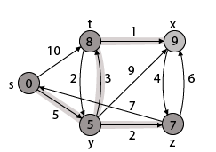
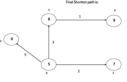
Thus, we get all shortest path vertex as
Weight from s to y is 5
Weight from s to z is 7
Weight from s to t is 8
Weight from s to x is 9
These are the shortest distance from the source's' in the given graph.
Disadvantage of Dijkstra's Algorithm:
- It does a blind search, so wastes a lot of time while processing.
- It can't handle negative edges.
- It leads to the acyclic graph and most often cannot obtain the right shortest path.
- We need to keep track of vertices that have been visited.
In Dijkstra’s algorithm, two sets are maintained, one set contains list of vertices already included in SPT (Shortest Path Tree), other set contains vertices not yet included. With adjacency list representation, all vertices of a graph can be traversed in O(V+E) time using BFS. The idea is to traverse all vertices of graph using BFS and use a Min Heap to store the vertices not yet included in SPT (or the vertices for which shortest distance is not finalized yet).
Min Heap is used as a priority queue to get the minimum distance vertex from set of not yet included vertices. Time complexity of operations like extract-min and decrease-key value is O(LogV) for Min Heap.
Following are the detailed steps.
1) Create a Min Heap of size V where V is the number of vertices in the given graph. Every node of min heap contains vertex number and distance value of the vertex.
2) Initialize Min Heap with source vertex as root (the distance value assigned to source vertex is 0). The distance value assigned to all other vertices is INF (infinite).
3) While Min Heap is not empty, do following
a) Extract the vertex with minimum distance value node from Min Heap. Let the extracted vertex be u.
b) For every adjacent vertex v of u, check if v is in Min Heap. If v is in Min Heap and distance value is more than weight of u-v plus distance value of u, then update the distance value of v.
Let us understand with the following example. Let the given source vertex be 0
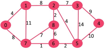
Initially, distance value of source vertex is 0 and INF (infinite) for all other vertices. So source vertex is extracted from Min Heap and distance values of vertices adjacent to 0 (1 and 7) are updated. Min Heap contains all vertices except vertex 0.
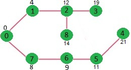
The vertices in green color are the vertices for which minimum distances are finalized and are not in Min Heap

Since distance value of vertex 1 is minimum among all nodes in Min Heap, it is extracted from Min Heap and distance values of vertices adjacent to 1 are updated (distance is updated if the vertex is in Min Heap and distance through 1 is shorter than the previous distance). Min Heap contains all vertices except vertex 0 and 1.
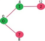
Pick the vertex with minimum distance value from min heap. Vertex 7 is picked. So min heap now contains all vertices except 0, 1 and 7. Update the distance values of adjacent vertices of 7. The distance value of vertex 6 and 8 becomes finite (15 and 9 respectively).
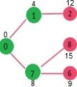
Pick the vertex with minimum distance from min heap. Vertex 6 is picked. So min heap now contains all vertices except 0, 1, 7 and 6. Update the distance values of adjacent vertices of 6. The distance value of vertex 5 and 8 are updated.
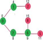
Above steps are repeated till min heap doesn’t become empty. Finally, we get the following shortest path tree.
Key takeaway
- Warshall’s algorithm constructs transitive closure of a given directed graph.
- In directed graphs there are n vertices.
- A graph with each edge directed is called a directed OR digraph graph.
- Dijkstra’s algorithm is the iterative algorithmic process to provide us with the shortest path from one specific starting node to all other nodes of a graph.
References:
1. Aaron M. Tenenbaum, Yedidyah Langsam and Moshe J. Augenstein, “Data Structures Using C and C++”, PHI Learning Private Limited, Delhi India
2. Horowitz and Sahani, “Fundamentals of Data Structures”, Galgotia Publications Pvt Ltd Delhi India.
3. Lipschutz, “Data Structures” Schaum’s Outline Series, Tata McGraw-hill Education (India) Pvt. Ltd.
4. Thareja, “Data Structure Using C” Oxford Higher Education.
5. AK Sharma, “Data Structure Using C”, Pearson Education India.