Unit – 5
Trees
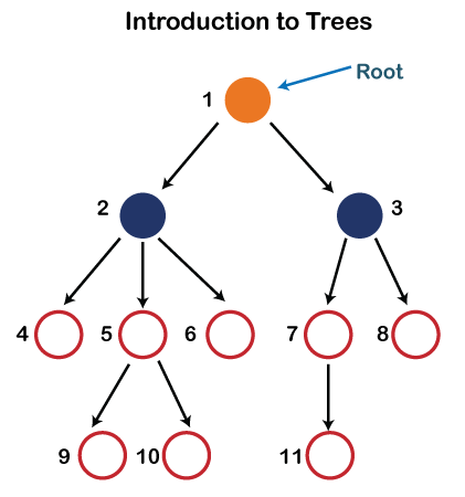
Fig 1: tree
Each node in the above structure is labeled with a number. Each arrow in the diagram above represents a link between the two nodes.
Root - In a tree hierarchy, the root node is the highest node. To put it another way, the root node is the one that has no children. The root node of the tree is numbered 1 in the above structure. A parent-child relationship exists when one node is directly linked to another node.
Child node - If a node is a descendant of another node, it is referred to as a child node.
Parent - If a node has a sub-node, the parent of that sub-node is said to be that node.
Sibling - Sibling nodes are those that have the same parent.
Leaf node - A leaf node is a node in the tree that does not have any descendant nodes. A leaf node is the tree's bottommost node. In a generic tree, there can be any number of leaf nodes. External nodes are also known as leaf nodes.
Internal node - An internal node is a node that has at least one child node.
Ancestor node - Any previous node on a path from the root to that node is an ancestor of that node. There are no ancestors for the root node. Nodes 1, 2, and 5 are the ancestors of node 10 in the tree depicted above.
Descendant node - A descendant of a node is the direct successor of the supplied node. In the diagram above, node 10 is a descendent of node 5.
Binary Tree
The Binary tree means that the node can have a maximum of two children. Here, binary name itself suggests 'two'; therefore, each node can have either 0, 1 or 2 children.
Let's understand the binary tree through an example.
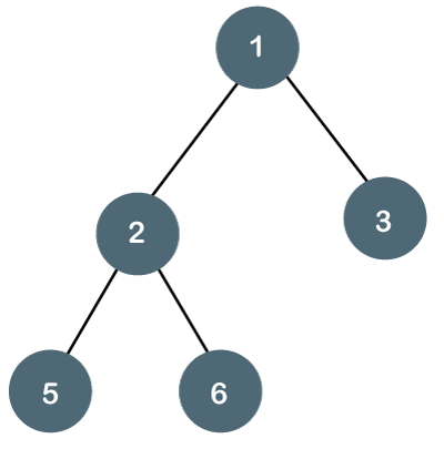
Fig 2 - Example
The above tree is a binary tree because each node contains the utmost two children. The logical representation of the above tree is given below:
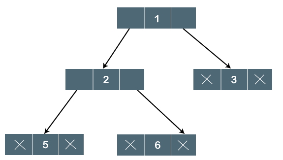
Fig 3 - logical representation
In the above tree, node 1 contains two pointers, i.e., left and a right pointer pointing to the left and right node respectively. The node 2 contains both the nodes (left and right node); therefore, it has two pointers (left and right). The nodes 3, 5 and 6 are the leaf nodes, so all these nodes contain NULL pointer on both left and right parts.
Properties of Binary Tree
● At each level of i, the maximum number of nodes is 2i.
● The height of the tree is defined as the longest path from the root node to the leaf node. The tree which is shown above has a height equal to 3. Therefore, the maximum number of nodes at height 3 is equal to (1+2+4+8) = 15. In general, the maximum number of nodes possible at height h is (20 + 21 + 22+….2h) = 2h+1 -1.
● The minimum number of nodes possible at height h is equal to h+1.
● If the number of nodes is minimum, then the height of the tree would be maximum. Conversely, if the number of nodes is maximum, then the height of the tree would be minimum.
If there are 'n' number of nodes in the binary tree.
The minimum height can be computed as:
As we know that,
n = 2h+1 -1
n+1 = 2h+1
Taking log on both the sides,
Log2(n+1) = log2(2h+1)
Log2(n+1) = h+1
h = log2(n+1) - 1
The maximum height can be computed as:
As we know that,
n = h+1
h= n-1
Types of Binary Tree
There are four types of Binary tree:
● Full/ proper/ strict Binary tree
● Complete Binary tree
● Perfect Binary tree
● Degenerate Binary tree
● Balanced Binary tree
Key takeaway
- The Binary tree means that the node can have a maximum of two children. Here, binary name itself suggests 'two'; therefore, each node can have either 0, 1 or 2 children.
There are two ways to express a binary tree data structure. The following are the techniques…
- Array Representation
- Linked List Representation
Array Representation
We utilize a one-dimensional array (1-D Array) to express a binary tree in an array representation.
Consider the binary tree shown above, which is represented as follows...
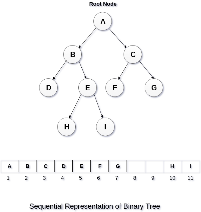
Fig 4: array representation
A one-dimensional array with a maximum size of 2n + 1 is required to represent a binary tree of depth 'n' using array representation.
Linked list Representation
A binary tree is represented as a double linked list. Every node in a double linked list has three fields. The left child address is stored in the first field, the actual data is stored in the second field, and the right child address is stored in the third field.
A node has the following structure in this linked list representation…

Example of the binary tree represented using Linked list representation is shown as follows…
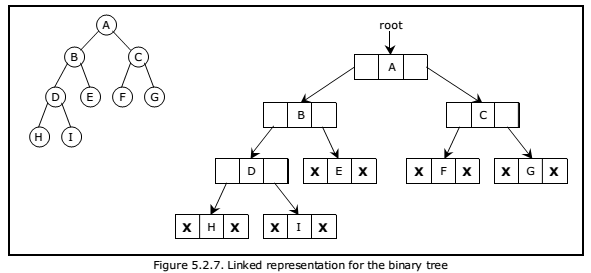
Fig 5: linked list representation
Key takeaway
- We utilize a one-dimensional array (1-D Array) to express a binary tree in an array representation.
- A binary tree is represented as a double linked list. Every node in a double linked list has three fields.
- The left child address is stored in the first field, the actual data is stored in the second field, and the right child address is stored in the third field.
A binary search tree is a type of binary tree in which the nodes are organized in a predetermined sequence. This is referred to as an ordered binary tree.
The value of all nodes in the left sub-tree is less than the value of the root in a binary search tree. Similarly, the value of all nodes in the right subtree is larger than or equal to the root's value. This rule will be applied recursively to all of the root's left and right subtrees.
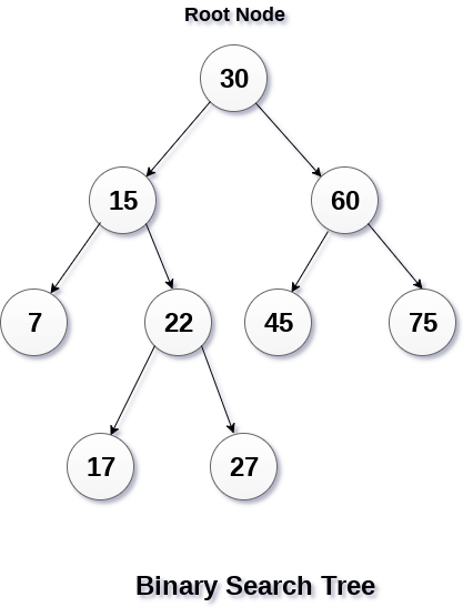
Fig 6: binary search tree
The image above depicts a binary search tree. We can see that the root node 30 doesn't have any values more than or equal to 30 in its left sub-tree, and it also doesn't have any values less than 30 in its right subtree, thanks to the restriction given to the BST.
Advantages
- In a binary search tree, searching becomes incredibly efficient since we get a hint at each step about which sub-tree has the sought element.
- In comparison to arrays and linked lists, the binary search tree is a more efficient data structure. Every stage of the search procedure destroys half of the sub-tree. In a binary search tree, searching for an element takes o(log2n) time.
- It also speeds up the insertion and deletion operations as compared to that in array and linked list.
Operation on binary search tree
Searching - In a binary search tree, finding the position of a certain element.
Insertion - Adding a new element to the binary search tree in the proper location to ensure that the BST property is not violated.
Deletion - In a binary search tree, removing a specific node. However, depending on the amount of children a node has, there can be a variety of deletion scenarios.
Key takeaway
- A binary search tree is a type of binary tree in which the nodes are organized in a predetermined sequence. This is referred to as an ordered binary tree.
- The value of all nodes in the left sub-tree is less than the value of the root in a binary search tree.
A strictly binary tree is one in which every non-leaf node in a binary tree has nonempty left and right subtrees. 2n -1 nodes are always present in a strictly binary tree with n leaves.
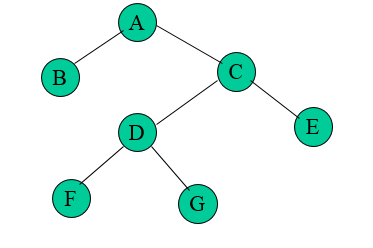
Fig 7: strict binary tree
A binary tree is said to be strictly binary if every non-leaf node contains nonempty left and right subtrees. To put it another way, in a purely binary tree, all nodes are of degree zero or two, never one.
A binary tree is a finite collection of elements that is either empty or divided into three distinct sections. The first subset has a single element known as the tree's root. The left and right subtrees of the original tree are binary trees, as are the other two subsets. It is possible for a left or right subtree to be empty.
A node of a binary tree is each of the tree's elements, and the tree has nine nodes with A as its root. The left subtree of this tree is rooted at B, whereas the right subtree is rooted at C. The two branches emerging from A to B on the left and to C on the right demonstrate this. An empty subtree is indicated by the lack of a branch.
The complete binary tree is a tree in which all the nodes are completely filled except the last level. In the last level, all the nodes must be as left as possible. In a complete binary tree, the nodes should be added from the left.
Let's create a complete binary tree.
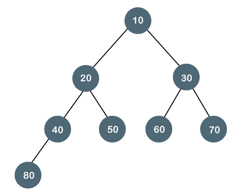
Fig 8 - Complete binary tree
The above tree is a complete binary tree because all the nodes are completely filled, and all the nodes in the last level are added at the left first.
Properties of Complete Binary Tree
● The maximum number of nodes in a complete binary tree is 2h+1 - 1.
● The minimum number of nodes in a complete binary tree is 2h.
● The minimum height of a complete binary tree is log2(n+1) - 1.
● The maximum height of a complete binary tree is
An extended binary tree is a sort of binary tree in which all of the original tree's null subtrees are replaced with special nodes known as external nodes, while other nodes are known as internal nodes.

Fig 9: extended binary tree
The internal nodes are represented by circles, whereas the external nodes are represented by boxes.
Properties
- Internal nodes are those from the original tree, whereas external nodes are those from the special tree.
- Internal nodes are non-leaf nodes, while all external nodes are leaf nodes.
- Every exterior node is a leaf, and every internal node has precisely two children. It shows the outcome, which is a full binary tree.
Traversal is a process to visit all the nodes of a tree and may print their values too. Because all nodes are connected via edges (links) we always start from the root (head) node. That is, we cannot randomly access a node in a tree. There are three ways which we use to traverse a tree −
● In-order Traversal
● Pre-order Traversal
● Post-order Traversal
Generally, we traverse a tree to search or locate a given item or key in the tree or to print all the values it contains.
In-order Traversal
In this traversal method, the left subtree is visited first, then the root and later the right sub-tree. We should always remember that every node may represent a subtree itself.
If a binary tree is traversed in-order, the output will produce sorted key values in an ascending order.
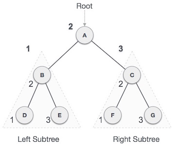
Fig 10 - Inorder
We start from A, and following in-order traversal, we move to its left subtree B. B is also traversed in-order. The process goes on until all the nodes are visited. The output of inorder traversal of this tree will be −
D → B → E → A → F → C → G
Algorithm
Until all nodes are traversed −
Step 1 − Recursively traverse left subtree.
Step 2 − Visit root node.
Step 3 − Recursively traverse right subtree.
Pre-order Traversal
In this traversal method, the root node is visited first, then the left subtree and finally the right subtree.
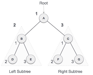
Fig 11 – Pre order
We start from A, and following pre-order traversal, we first visit A itself and then move to its left subtree B. B is also traversed pre-order. The process goes on until all the nodes are visited. The output of pre-order traversal of this tree will be −
A → B → D → E → C → F → G
Algorithm
Until all nodes are traversed −
Step 1 − Visit root node.
Step 2 − Recursively traverse left subtree.
Step 3 − Recursively traverse right subtree.
Post-order Traversal
In this traversal method, the root node is visited last, hence the name. First, we traverse the left subtree, then the right subtree and finally the root node.
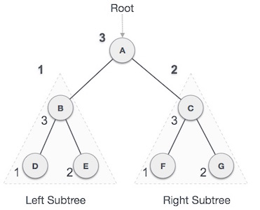
Fig 12 – Post order
We start from A, and following Post-order traversal, we first visit the left subtree B. B is also traversed post-order. The process goes on until all the nodes are visited. The output of post-order traversal of this tree will be −
D → E → B → F → G → C → A
Algorithm
Until all nodes are traversed −
Step 1 − Recursively traverse left subtree.
Step 2 − Recursively traverse right subtree.
Step 3 − Visit root node.
Tree Traversal in C
Traversal is a process to visit all the nodes of a tree and may print their values too. Because, all nodes are connected via edges (links) we always start from the root (head) node. That is, we cannot random access a node in a tree. There are three ways which we use to traverse a tree −
● In-order Traversal
● Pre-order Traversal
● Post-order Traversal
We shall now look at the implementation of tree traversal in C programming language here using the following binary tree −
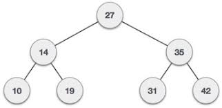
Fig 13 - Example
Implementation in C
#include <stdio.h>
#include <stdlib.h>
Struct node {
Int data;
Struct node *leftChild;
Struct node *rightChild;
};
Struct node *root = NULL;
Void insert(int data) {
Struct node *tempNode = (struct node*) malloc(sizeof(struct node));
Struct node *current;
Struct node *parent;
TempNode->data = data;
TempNode->leftChild = NULL;
TempNode->rightChild = NULL;
//if tree is empty
If(root == NULL) {
Root = tempNode;
} else {
Current = root;
Parent = NULL;
While(1) {
Parent = current;
//go to left of the tree
If(data < parent->data) {
Current = current->leftChild;
//insert to the left
If(current == NULL) {
Parent->leftChild = tempNode;
Return;
}
} //go to right of the tree
Else {
Current = current->rightChild;
//insert to the right
If(current == NULL) {
Parent->rightChild = tempNode;
Return;
}
}
}
}
}
Struct node* search(int data) {
Struct node *current = root;
Printf("Visiting elements: ");
While(current->data != data) {
If(current != NULL)
Printf("%d ",current->data);
//go to left tree
If(current->data > data) {
Current = current->leftChild;
}
//else go to right tree
Else {
Current = current->rightChild;
}
//not found
If(current == NULL) {
Return NULL;
}
}
Return current;
}
Void pre_order_traversal(struct node* root) {
If(root != NULL) {
Printf("%d ",root->data);
Pre_order_traversal(root->leftChild);
Pre_order_traversal(root->rightChild);
}
}
Void inorder_traversal(struct node* root) {
If(root != NULL) {
Inorder_traversal(root->leftChild);
Printf("%d ",root->data);
Inorder_traversal(root->rightChild);
}
}
Void post_order_traversal(struct node* root) {
If(root != NULL) {
Post_order_traversal(root->leftChild);
Post_order_traversal(root->rightChild);
Printf("%d ", root->data);
}
}
Int main() {
Int i;
Int array[7] = { 27, 14, 35, 10, 19, 31, 42 };
For(i = 0; i < 7; i++)
Insert(array[i]);
i = 31;
Struct node * temp = search(i);
If(temp != NULL) {
Printf("[%d] Element found.", temp->data);
Printf("\n");
}else {
Printf("[ x ] Element not found (%d).\n", i);
}
i = 15;
Temp = search(i);
If(temp != NULL) {
Printf("[%d] Element found.", temp->data);
Printf("\n");
}else {
Printf("[ x ] Element not found (%d).\n", i);
}
Printf("\nPreorder traversal: ");
Pre_order_traversal(root);
Printf("\nInorder traversal: ");
Inorder_traversal(root);
Printf("\nPost order traversal: ");
Post_order_traversal(root);
Return 0;
}
If we compile and run the above program, it will produce the following result −
Output
Visiting elements: 27 35 [31] Element found.
Visiting elements: 27 14 19 [ x ] Element not found (15).
Preorder traversal: 27 14 10 19 35 31 42
Inorder traversal: 10 14 19 27 31 35 42
Post order traversal: 10 19 14 31 42 35 27
Key takeaway
- Traversal is a process to visit all the nodes of a tree and may print their values too.
- Because all nodes are connected via edges (links) we always start from the root (head) node.
- In this traversal method, the left subtree is visited first, then the root and later the right subtree.
- Post order traversal method, the root node is visited last, hence the name. First, we traverse the left subtree, then the right subtree and finally the root node.
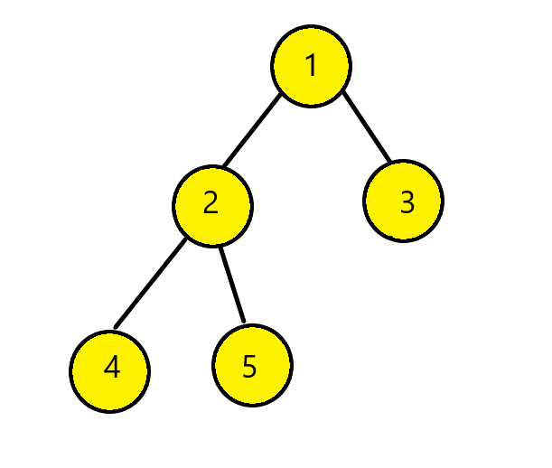
Inorder Traversal: [4, 2, 5, 1, 3]
Postorder Traversal: [4, 5, 2, 3, 1]
The rightmost element, node 1, is now the root node, as we can see from the post order traversal. We can see that node 3 is to the right of root node 1, while others are on the left, thanks to inorder traversal.
In a similar manner, we arrive at tree:
The insertion operation in a binary search tree takes O(log n) time to complete. A new node is always added as a leaf node in a binary search tree. The following is how the insertion procedure is carried out...
Step 1: Create a newNode with the specified value and NULL left and right.
Step 2: Make sure the tree isn't empty.
Step 3 - Set root to newNode if the tree is empty.
Step 4 - If the tree isn't empty, see if newNode's value is smaller or larger than the node's value (here it is root node).
Step 5 - Go to the node's left child if newNode is smaller or equal to it. Move to newNode's right child if newNode is larger than the node.
Step 6- Continue in this manner until we reach the leaf node (i.e., reaches to NULL).
Step 7 - Once you've reached the leaf node, insert the newNode as a left child if it's smaller or equal to the leaf node, or as a right child otherwise.
Deletion
The deletion process in a binary search tree takes O(log n) time to complete. The three scenarios for removing a node from a Binary search tree are as follows...
Case 1: Deleting a Leaf node (A node with no children)
Case 2: Deleting a node with one child
Case 3: Deleting a node with two children
Case 1: Deleting a Leaf node
To delete a leaf node from BST, follow these steps...
Step 1: Using the search function, locate the node to be eliminated.
Step 2 - If the node is a leaf, delete it with the free function and end the function.
Case 2: Deleting a node with one child
To delete a node with one child from BST, we utilize the procedures below...
Step 1: Using the search function, locate the node to be eliminated.
Step 2 - Create a link between the parent node and the child node if it only has one child.
Step 3: Using the free function, delete the node and exit the function
Case 3: Deleting a node with two children
To delete a node with two children from BST, we utilize the procedures below...
Step 1: Using the search function, locate the node to be eliminated.
Step 2 - Find the largest node in the left subtree (OR the smallest node in the right subtree) if it has two children.
Step 3 - Swap the deleting node with the node discovered in the previous step.
Step 4 - Next, see if deleting the node resulted in case 1 or case 2, if not, move to step 2.
Step 5 - If case 1 applies, delete it using case 1 reasoning.
Step 6- If case 2 applies, delete it using case 2 reasoning.
Step 7 - Continue in this manner until the node has been removed from the tree.
Searching
The search operation in a binary search tree takes O(log n) time to complete. The following is how the search is carried out...
Step 1: Ask the user for the search element.
Step 2: Compare the value of the root node in the tree to the search element.
Step 3 - If both matches, the function will display "Given node is found!!!" and the function will be terminated.
Step 4 - If neither of the search elements match, see if the search element is smaller or larger than the node value.
Step 5 - Continue searching in the left subtree if the search element is smaller.
Step 6- If the search element is larger, move on to the correct subtree and continue the search.
Step 7 - Continue in this manner until the exact element is found or the search element is compared to the leaf node.
Step 8 - If we reach a node with a value equal to the search value, we'll get "Element found" and the function will end.
Step 9 - If we get to the leaf node and it doesn't match the search element, we'll see "Element not found" and the function will end.
Example
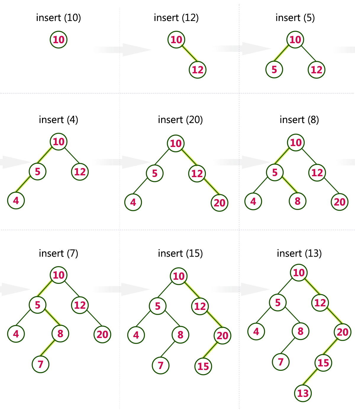
Create a Binary Search Tree by adding the integers in the following order…
10,12,5,4,20,8,7,15 and 13
The following items are added into a Binary Search Tree in the following order...
Here we will see the threaded binary tree data structure. We know that the binary tree nodes may have at most two children. But if they have only one child, or no children, the link part in the linked list representation remains null. Using threaded binary tree representation, we can reuse that empty link by making some threads.
If one node has some vacant left or right child area, that will be used as thread. There are two types of threaded binary tree. The single threaded tree or fully threaded binary tree. In single threaded mode, there are another two variations. Left threaded and right threaded.
In the left threaded mode if some node has no left child, then the left pointer will point to its inorder predecessor, similarly in the right threaded mode if some node has no right child, then the right pointer will point to its inorder successor. In both cases, if no successor or predecessor is present, then it will point to the header node.
For fully threaded binary tree, each node has five fields. Three fields like normal binary tree node, another two fields to store Boolean value to denote whether link of that side is actual link or thread.
Left Thread Flag Left Link Data Right Link Right Thread Flag
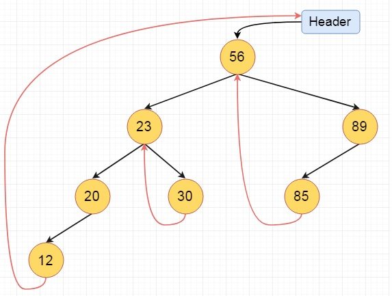
Fig 14 - Example
These are the examples of left and right threaded tree
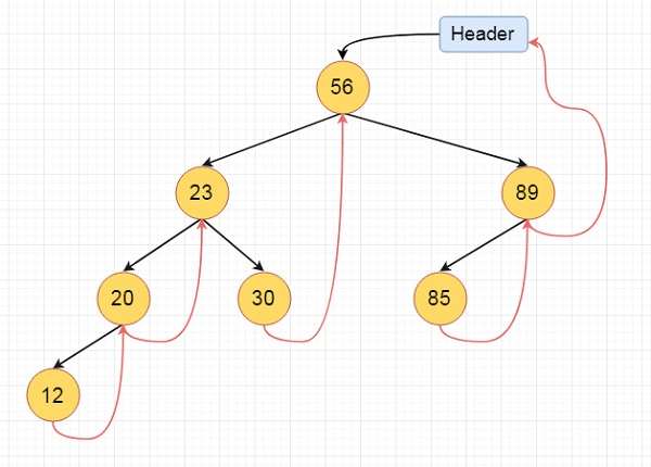
Fig 15 - Example
This is the fully threaded binary tree
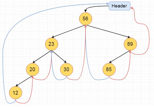
Fig 16 - Fully threaded binary tree
Key takeaway
- Here we will see the threaded binary tree data structure. We know that the binary tree nodes may have at most two children.
- But if they have only one child, or no children, the link part in the linked list representation remains null.
- Using threaded binary tree representation, we can reuse that empty links by making some threads.
If one node has some vacant left or right child area, that will be used as thread. There are two types of threaded binary tree. The single threaded tree or fully threaded binary tree. In single threaded mode, there are another two variations. Left threaded and right threaded.
The binary tree nodes can only have two children, according to our knowledge. However, if they only have one child or none at all, the link component of the linked list representation is null. We can reuse those empty links by creating threads using threaded binary tree representation.
If a node's left or right child area is empty, it will be used as a thread. A threaded binary tree can be divided into two categories. The binary tree is either a single threaded tree or a fully threaded binary tree.
Each node in a fully threaded binary tree has five fields. Three fields, one for each node in a binary tree, and two more for storing a Boolean value indicating whether the link on that side is an actual link or a thread.
Left Thread Flag | Left Link | Data | Right Link | Right Thread Flag |
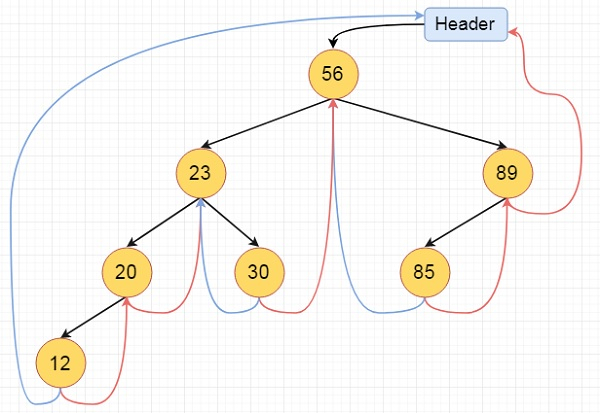
Fig 17: fully threaded binary tree
Algorithm
Inorder():
Begin
Temp:= root
Repeat infinitely, do
p:= temp
Temp = right of temp
If right flag of p is false, then
While left flag of temp is not null, do
Temp:= left of temp
Done
End if
If temp and root are same, then
Break
End if
Print key of temp
Done
End
Characters are coded using Huffman coding, and the length of the code is determined by the relative frequency or weight of the associated character. Huffman codes come in a variety of lengths and don't have any prefixes (that means no code is a prefix of any other). Any prefix-free binary code can be represented as a binary tree, with the encoded characters at the leaves.
The Huffman tree, also known as the Huffman coding tree, is a full binary tree in which each leaf corresponds to a letter in the alphabet.
The Huffman tree is regarded as the binary tree with the smallest external path weight, i.e., the one with the smallest sum of weighted path lengths for a given set of leaves. As a result, the goal is to build a tree with the least amount of external path weight.
The following is an example:
Letter frequency table
Letter | z | k | m | c | u | d | l | e |
Frequency | 2 | 7 | 24 | 32 | 37 | 42 | 42 | 120 |
Huffman code
Letter | Freq | Code | Bits |
e | 120 | 0 | 1 |
d | 42 | 101 | 3 |
l | 42 | 110 | 3 |
u | 37 | 100 | 3 |
c | 32 | 1110 | 4 |
m | 24 | 11111 | 5 |
k | 7 | 111101 | 6 |
z | 2 | 111100 | 6 |
The Huffman tree (for the above example) is given below -
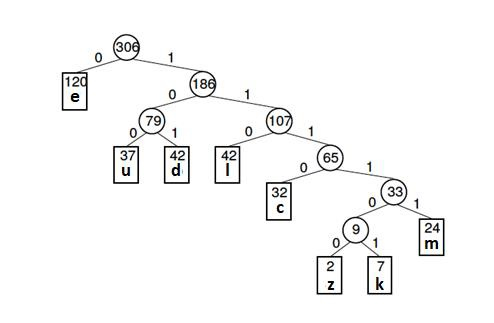
Fig 18: Huffman tree
Key takeaway
- Characters are coded using Huffman coding, and the length of the code is determined by the relative frequency or weight of the associated character.
- Huffman codes come in a variety of lengths and don't have any prefixes.
AVL Tree was invented by GM Adelson - Velsky and EM Landis in 1962. The tree is named AVL in honour of its inventors.
AVL Tree can be defined as a height balanced binary search tree in which each node is associated with a balance factor which is calculated by subtracting the height of its right subtree from that of its left sub-tree.
Tree is said to be balanced if the balance factor of each node is in between -1 to 1, otherwise, the tree will be unbalanced and need to be balanced.
Balance Factor (k) = height (left(k)) - height (right(k))
If balance factor of any node is 1, it means that the left sub-tree is one level higher than the right subtree.
If balance factor of any node is 0, it means that the left subtree and right subtree contain equal height.
If balance factor of any node is -1, it means that the left sub-tree is one level lower than the right subtree.
An AVL tree is given in the following figure. We can see that, balance factor associated with each node is in between -1 and +1. Therefore, it is an example of AVL tree.
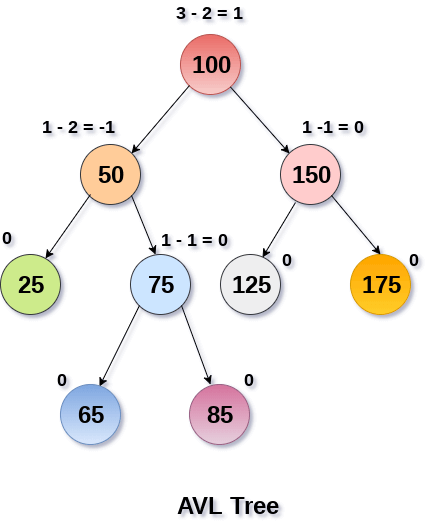
Fig 19: AVL Tree
Complexity
Algorithm | Average case | Worst case |
Space | o(n) | o(n) |
Search | o(log n) | o(log n) |
Insert | o(log n) | o(log n) |
Delete | o(log n) | o(log n) |
Operations on AVL tree
Due to the fact that, AVL tree is also a binary search tree therefore, all the operations are performed in the same way as they are performed in a binary search tree. Searching and traversing do not lead to the violation in property of AVL tree. However, insertion and deletion are the operations which can violate this property and therefore, they need to be revisited.
SN | Operation | Description |
1 | Insertion | Insertion in AVL tree is performed in the same way as it is performed in a binary search tree. However, it may lead to violation in the AVL tree property and therefore the tree may need balancing. The tree can be balanced by applying rotations. |
2 | Deletion | Deletion can also be performed in the same way as it is performed in a binary search tree. Deletion may also disturb the balance of the tree therefore, various types of rotations are used to rebalance the tree. |
Why AVL Tree?
AVL tree controls the height of the binary search tree by not letting it to be skewed. The time taken for all operations in a binary search tree of height h is O(h). However, it can be extended to O(n) if the BST becomes skewed (i.e., worst case). By limiting this height to log n, AVL tree imposes an upper bound on each operation to be O(log n) where n is the number of nodes.
AVL Rotations
We perform rotation in AVL tree only in case if Balance Factor is other than -1, 0, and 1. There are basically four types of rotations which are as follows:
- L L rotation: Inserted node is in the left subtree of left subtree of A
- R R rotation: Inserted node is in the right subtree of right subtree of A
- L R rotation: Inserted node is in the right subtree of left subtree of A
- R L rotation: Inserted node is in the left subtree of right subtree of A
Where node A is the node whose balance Factor is other than -1, 0, 1.
The first two rotations LL and RR are single rotations and the next two rotations LR and RL are double rotations. For a tree to be unbalanced, minimum height must be at least 2, Let us understand each rotation
1. RR Rotation
When BST becomes unbalanced, due to a node is inserted into the right subtree of the right subtree of A, then we perform RR rotation, RR rotation is an anticlockwise rotation, which is applied on the edge below a node having balance factor -2
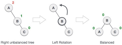
In above example, node A has balance factor -2 because a node C is inserted in the right subtree of A right subtree. We perform the RR rotation on the edge below A.
2. LL Rotation
When BST becomes unbalanced, due to a node is inserted into the left subtree of the left subtree of C, then we perform LL rotation, LL rotation is clockwise rotation, which is applied on the edge below a node having balance factor 2.
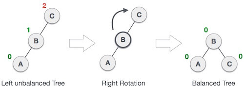
In above example, node C has balance factor 2 because a node A is inserted in the left subtree of C left subtree. We perform the LL rotation on the edge below A.
3. LR Rotation
Double rotations are bit tougher than single rotation which has already explained above. LR rotation = RR rotation + LL rotation, i.e., first RR rotation is performed on subtree and then LL rotation is performed on full tree, by full tree we mean the first node from the path of inserted node whose balance factor is other than -1, 0, or 1.
Let us understand each and every step very clearly:
State | Action |
| A node B has been inserted into the right subtree of A the left subtree of C, because of which C has become an unbalanced node having balance factor 2. This case is L R rotation where: Inserted node is in the right subtree of left subtree of C |
| As LR rotation = RR + LL rotation, hence RR (anticlockwise) on subtree rooted at A is performed first. By doing RR rotation, node A, has become the left subtree of B. |
| After performing RR rotation, node C is still unbalanced, i.e., having balance factor 2, as inserted node A is in the left of left of C |
| Now we perform LL clockwise rotation on full tree, i.e., on node C. Node C has now become the right subtree of node B, A is left subtree of B |
| Balance factor of each node is now either -1, 0, or 1, i.e., BST is balanced now. |
4. RL Rotation
As already discussed, that double rotations are bit tougher than single rotation which has already explained above. R L rotation = LL rotation + RR rotation, i.e., first LL rotation is performed on subtree and then RR rotation is performed on full tree, by full tree we mean the first node from the path of inserted node whose balance factor is other than -1, 0, or 1.
State | Action |
| A node B has been inserted into the left subtree of C the right subtree of A, because of which A has become an unbalanced node having balance factor - 2. This case is RL rotation where: Inserted node is in the left subtree of right subtree of A |
| As RL rotation = LL rotation + RR rotation, hence, LL (clockwise) on subtree rooted at C is performed first. By doing RR rotation, node C has become the right subtree of B. |
| After performing LL rotation, node A is still unbalanced, i.e., having balance factor -2, which is because of the right-subtree of the right-subtree node A. |
| Now we perform RR rotation (anticlockwise rotation) on full tree, i.e., on node A. Node C has now become the right subtree of node B, and node A has become the left subtree of B. |
| Balance factor of each node is now either -1, 0, or 1, i.e., BST is balanced now. |
Q: Construct an AVL tree having the following elements
H, I, J, B, A, E, C, F, D, G, K, L
1. Insert H, I, J
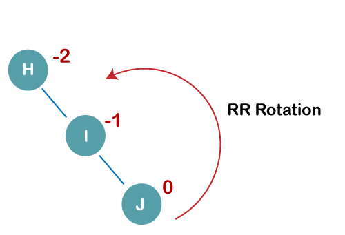
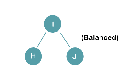
On inserting the above elements, especially in the case of H, the BST becomes unbalanced as the Balance Factor of H is -2. Since the BST is right-skewed, we will perform RR Rotation on node H.
The resultant balance tree is:
2. Insert B, A
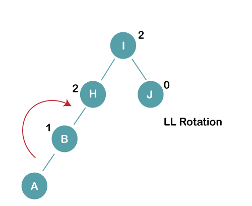
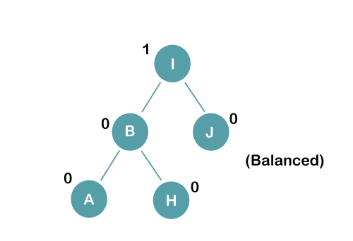
On inserting the above elements, especially in case of A, the BST becomes unbalanced as the Balance Factor of H and I is 2, we consider the first node from the last inserted node i.e., H. Since the BST from H is left-skewed, we will perform LL Rotation on node H.
The resultant balance tree is:
3. Insert E
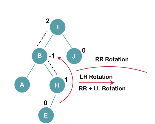
On inserting E, BST becomes unbalanced as the Balance Factor of I is 2, since if we travel from E to I we find that it is inserted in the left subtree of right subtree of I, we will perform LR Rotation on node I. LR = RR + LL rotation
3 a) We first perform RR rotation on node B
The resultant tree after RR rotation is:
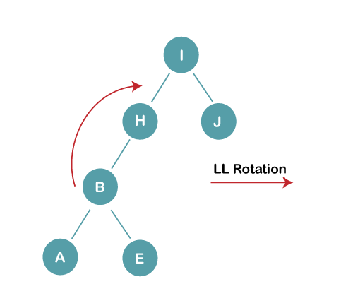
3b) We first perform LL rotation on the node I
The resultant balanced tree after LL rotation is:
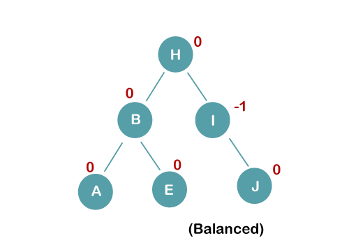
4. Insert C, F, D
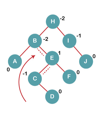
On inserting C, F, D, BST becomes unbalanced as the Balance Factor of B and H is -2, since if we travel from D to B, we find that it is inserted in the right subtree of left subtree of B, we will perform RL Rotation on node I. RL = LL + RR rotation.
4a) We first perform LL rotation on node E
The resultant tree after LL rotation is:
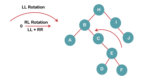
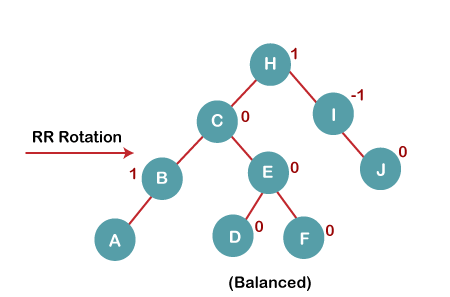
4b) We then perform RR rotation on node B
The resultant balanced tree after RR rotation is:
5. Insert G
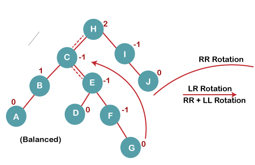
On inserting G, BST become unbalanced as the Balance Factor of H is 2, since if we travel from G to H, we find that it is inserted in the left subtree of right subtree of H, we will perform LR Rotation on node I. LR = RR + LL rotation.
5 a) We first perform RR rotation on node C
The resultant tree after RR rotation is:
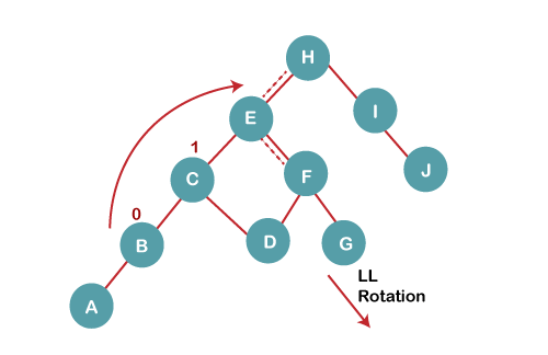
5 b) We then perform LL rotation on node H
The resultant balanced tree after LL rotation is:
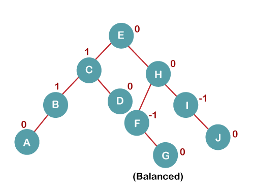
6. Insert K
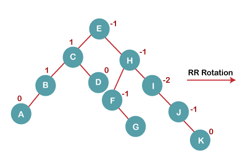
On inserting K, BST becomes unbalanced as the Balance Factor of I is -2. Since the BST is right-skewed from I to K, hence we will perform RR Rotation on the node I.
The resultant balanced tree after RR rotation is:
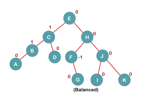
7. Insert L
On inserting the L tree is still balanced as the Balance Factor of each node is now either, -1, 0, +1. Hence the tree is a Balanced AVL tree
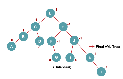
Key takeaway
- AVL Tree was invented by GM Adelson - Velsky and EM Landis in 1962. The tree is named AVL in honour of its inventors.
- AVL Tree can be defined as height balanced binary search tree in which each node is associated with a balance factor which is calculated by subtracting the height of its right sub-tree from that of its left sub-tree.
- Tree is said to be balanced if balance factor of each node is in between -1 to 1, otherwise, the tree will be unbalanced and need to be balanced.
An extended binary tree is a sort of binary tree in which all of the original tree's null subtrees are replaced with special nodes known as external nodes, while other nodes are known as internal nodes.
The internal nodes are represented by circles, whereas the external nodes are represented by boxes.
- Internal nodes are those from the original tree, whereas external nodes are those from the special tree.
- Internal nodes are non-leaf nodes, while all external nodes are leaf nodes.
- Every exterior node is a leaf, and every internal node has precisely two children.
- It shows the outcome, which is a full binary tree.
It is not required that all nodes have the same number of children, but each node must include m/2 nodes.
The following graphic depicts a B tree of order 4.
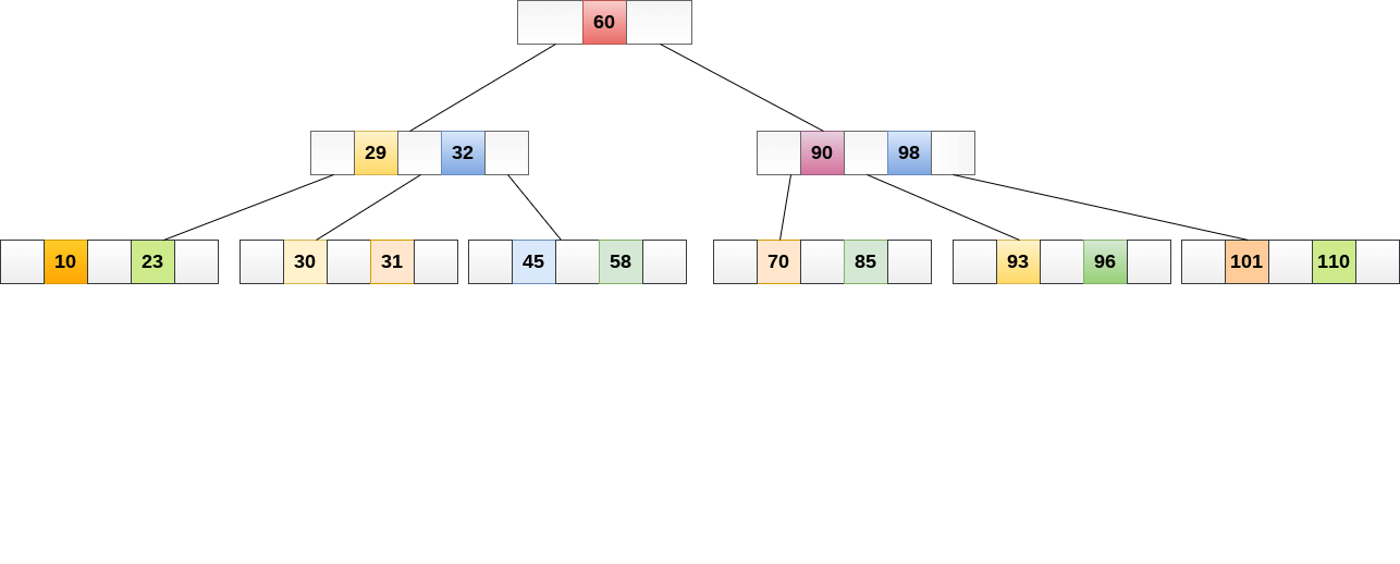
Fig 20: B tree
Any attribute of B Tree may be violated while performing some operations on it, such as the number of minimum children a node can have. The tree may split or unite in order to keep the features of B Tree.
Application of B tree
Because accessing values held in a huge database that is saved on a disk is a very time-consuming activity, B tree is used to index the data and enable fast access to the actual data stored on the disks.
In the worst situation, searching an unindexed and unsorted database with n key values takes O(n) time. In the worst-case scenario, if we use B Tree to index this database, it will be searched in O (log n) time.
Operations
Searching
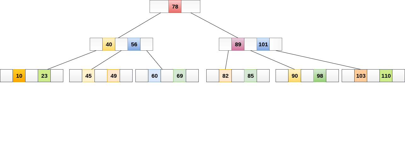
B Trees are comparable to Binary Search Trees in terms of searching. For example, let's look for item 49 in the B Tree below. The procedure will go somewhat like this:
- Compare item 49 to node 78, which is the root node. Move to the left sub-tree since 49 78 onwards.
- Since 404956, move to the right sub-tree of 40. 49>45, move to the right sub-tree of 40.
- Compare and contrast 49.
- Return if a match is found.
The height of the tree affects the search in a B tree. To search any element in a B tree, the search technique requires O (log n) time.
Inserting
At the leaf node level, insertions are made. In order to place an item into B Tree, the following algorithm must be followed.
- Navigate the B Tree until you find the suitable leaf node to insert the node at.
- If there are fewer than m-1 keys in the leaf node, insert the element in ascending order.
- Otherwise, if the leaf node contains m-1 keys, proceed to the next step.
● In the rising sequence of elements, add the new element.
● At the middle, divide the node into two nodes.
● The median element should be pushed up to its parent node.
● If the parent node has the same m-1 number of keys as the child node, split it as well.
Deletion
At the leaf nodes, deletion is also conducted. It can be a leaf node or an inside node that needs to be destroyed. In order to delete a node from a B tree, use the following algorithm.
- Locate the leaf node.
- If the leaf node has more than m/2 keys, delete the required key from the node.
- If the leaf node lacks m/2 keys, fill in the gaps with the element from the eighth or left sibling.
● If the left sibling has more than m/2 elements, shift the intervening element down to the node where the key is deleted and push the largest element up to its parent.
● If the right sibling has more than m/2 items, shift the intervening element down to the node where the key is deleted and push the smallest element up to the parent.
4. Create a new leaf node by merging two leaf nodes and the parent node's intervening element if neither sibling has more than m/2 elements. If the parent has less than m/2 nodes, repeat the operation on the parent as well.
5. If the node to be destroyed is an internal node, its in-order successor or predecessor should be used instead. The process will be same as the node is deleted from the leaf node because the successor or predecessor will always be on the leaf node.
Binary Heap
A binary heap is a data structure that resembles a complete binary tree in appearance. The ordering features of the heap data structure are explained here. A Heap is often represented by an array. We'll use H to represent a heap.
Because the elements of a heap are kept in an array, the position of the parent node of the ith element can be located at i/2 if the starting index is 1. Position 2i and 2i + 1 are the left and right children of the ith node, respectively.
Based on the ordering property, a binary heap can be classed as a max-heap or a min-heap.
Max Heap
A node's key value is larger than or equal to the key value of the highest child in this heap.
Hence, H[Parent(i)] ≥ H[i]
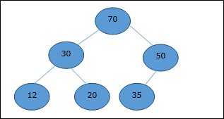
Fig 21: max heap
Min Heap
In mean-heap, a node's key value is less than or equal to the lowest child's key value.
Hence, H[Parent(i)] ≤ H[i]
Basic operations with respect to Max-Heap are shown below in this context. The insertion and deletion of elements in and out of heaps necessitates element reordering. As a result, the Heapify function must be used.
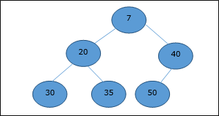
Fig 22: min heap
Key takeaway
- An extended binary tree is a sort of binary tree in which all of the original tree's null subtrees are replaced with special nodes known as external nodes, while other nodes are known as internal nodes.
- A binary heap is a data structure that resembles a complete binary tree in appearance.
- The ordering features of the heap data structure are explained here. A Heap is often represented by an array.
References:
1. Aaron M. Tenenbaum, Yedidyah Langsam and Moshe J. Augenstein, “Data Structures Using C and C++”, PHI Learning Private Limited, Delhi India
2. Horowitz and Sahani, “Fundamentals of Data Structures”, Galgotia Publications Pvt Ltd Delhi India.
3. Lipschutz, “Data Structures” Schaum’s Outline Series, Tata McGraw-hill Education (India) Pvt. Ltd.
4. Thareja, “Data Structure Using C” Oxford Higher Education.
5. AK Sharma, “Data Structure Using C”, Pearson Education India.