Unit – 3

Divide and Conquer

3.1 Divide and Conquer with Examples Such as Sorting

Divide & conquer is an efficient algorithm. It follows three steps: 

●      DIVIDE: divide problem into subproblems

●      RECUR:  Solve each sub problem recursively

●      CONQUER: Combine all solutions of sub problem to get original solution

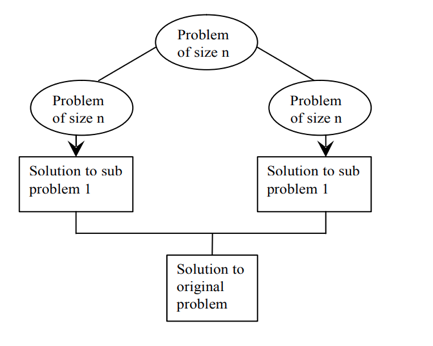
Fig 1: Divide and conquer plan

Advantages of divide and conquer

●      Divide to overcome conceptually challenging issues like Tower of Hanoi, Divide & Conquering is a versatile instrument.

●      Results with powerful algorithms

●      The algorithms of Divide & Conquer are adapted to the execution of enemies in multi-processors Machines

●      Results for algorithms that effectively use memory cache.

Disadvantages of divide and conquer

●      Recursions are sluggish,

●      It could be more complex than an iterative approach to a very simple problem.

Example: n numbers added etc.

Example

We divide a problem into two halves and solve each half separately using this method. After discovering the solution to each half, we combine them to reflect the main problem's solution.

Assume we have an array A, and our main objective is to sort the subsection represented by A[p..r], which starts at index p and ends at index r.

Divide

If q is believed to be the central point between p and r, the subarray A[p..r] will be split into two arrays, A[p..q] and A[q+1, r].

Conquer

The next stage is to conquer after splitting the arrays into two parts. Both the subarrays A[p..q] and A[q+1, r] are individually sorted in this phase. In case if we did not reach the base situation, then we again follow the same procedure, i.e., we further segment these subarrays followed by sorting them separately.

Combine

We successfully receive our sorted subarrays A[p..q] and A[q+1, r] when the conquer step acquires the base step, and then we combine them back to build a new sorted array [p..r].

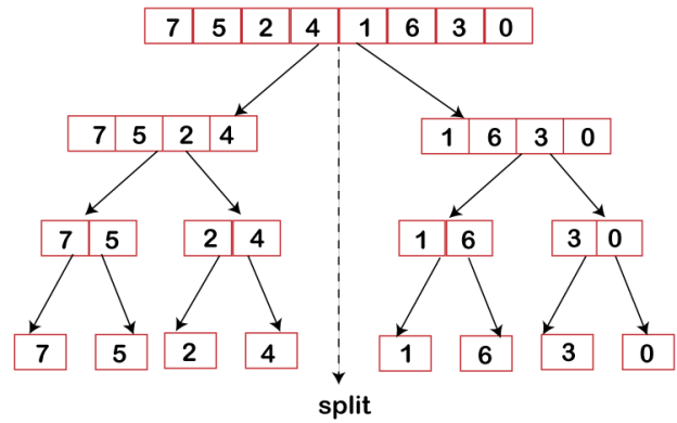
Fig 2: Merge sort divide phase

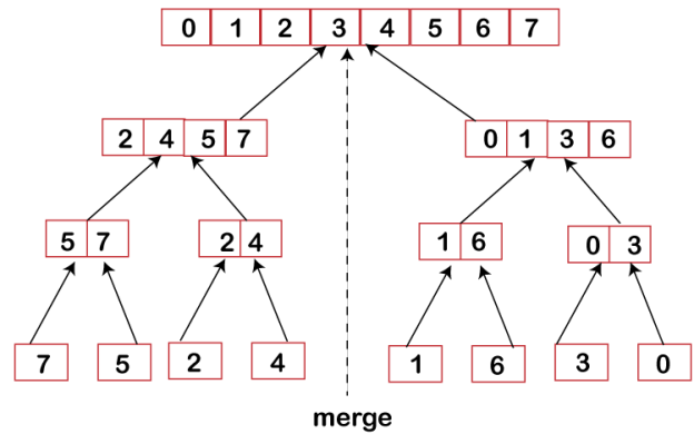
Fig 3: Merge sort combine phase

Key takeaway

1. DIVIDE: divide problem into subproblems
2. RECUR:  Solve each sub problem recursively
3. CONQUER: Combine all solutions of sub problem to get original solution

3.2 Matrix Multiplication

The standard method of matrix multiplication of two n x n matrices takes T(n) = O(n3).

The following algorithm multiplies nxn matrices A and B:

// Initialize C.

For i = 1 to n

For j = 1 to n

For k = 1 to n

C [i, j] += A[i, k] * B[k, j];

Strassen’s algorithm is a Divide-and-Conquer algorithm that beats the bound. The usual multiplication of two n x n matrices takes

If C=AB, then we have the following:

c11 = a11 b11 + a12 b21

c12 = a11 b12 + b12 b22

c21 = a21 b11 + a22 b21

c22 = a21 b12 + a22 b22  

8     n/2 * n/2 matrix multiples plus

4     n/2 * n/2 matrix additions

T(n) = 8T(n/2) + O(n2)

Plug in       a = 8, b = 2, k = 2 →logba=3    →   T(n)= O(n3)

Strassen showed how two matrices can be multiplied using only 7 multiplications and 18 additions:

Consider calculating the following 7 products:

q1 = (a11 + a22) * (b11 + b22)

q2 = (a21 + a22) * b11

q3 = a11*(b12 – b22)

q4 = a22 * (b21 – b11)

q5 = (a11 + a12) * b22

q6 = (a21 – a11) * (b11 + b12)

q7 = (a12 – a22) * (b21 + b22)

It turns out that

c11 = q1 + q4 – q5 + q7

c12 = q3 + q5

c21 = q2 + q4

c22 = q1 + q3 – q2 + q6

Code for Implementation of Strassen’s Matrix Multiplication

#include <assert.h>

#include <stdio.h>

#include <stdlib.h>

#include <time.h>

#define M 2

#define N (1<<M)

Typedef double datatype;

#define DATATYPE_FORMAT "%4.2g"

Typedef datatype mat[N][N];

Typedef struct

{

Intra, rb, ca, cb;

} corners;

Void identity(mat A, corners a)

{

Int i, j;

For (i = a.ra; i<a.rb; i++)

For (j = a.ca; j <a.cb; j++)

A[i][j] = (datatype) (i == j);

}

Void set(mat A, corners a, datatype k)

{

Int i, j;

For (i = a.ra; i<a.rb; i++)

For (j = a.ca; j <a.cb; j++)

A[i][j] = k;

}

Voidrandk(mat A, corners a, double l, double h)

{

Int i, j;

For (i = a.ra; i<a.rb; i++)

For (j = a.ca; j <a.cb; j++)

A[i][j] = (datatype) (l + (h - l) * (rand() / (double) RAND_MAX));

}

Void print(mat A, corners a, char *name)

{

Int i, j;

Printf("%s = {\n", name);

For (i = a.ra; i<a.rb; i++)

{

For (j = a.ca; j <a.cb; j++)

Printf(DATATYPE_FORMAT ", ", A[i][j]);

Printf("\n");

}

Printf("}\n");

}

Void add(mat A, mat B, mat C, corners a, corners b, corners c)

{

Intrd = a.rb - a.ra;

Int cd = a.cb - a.ca;

Int i, j;

For (i = 0; i<rd; i++)

{

For (j = 0; j < cd; j++)

{

C[i + c.ra][j + c.ca] = A[i + a.ra][j + a.ca] + B[i + b.ra][j

+ b.ca];

}

}

}

Void sub(mat A, mat B, mat C, corners a, corners b, corners c)

{

Intrd = a.rb - a.ra;

Int cd = a.cb - a.ca;

Int i, j;

For (i = 0; i<rd; i++)

{

For (j = 0; j < cd; j++)

{

C[i + c.ra][j + c.ca] = A[i + a.ra][j + a.ca] - B[i + b.ra][j

+ b.ca];

} }

}

Voidfind_corner(corners a, inti, int j, corners *b)

{

Intrm = a.ra + (a.rb - a.ra) / 2;

Int cm = a.ca + (a.cb - a.ca) / 2;

*b = a;

If (i == 0)

b->rb = rm;

Else

b->ra = rm;

If (j == 0)

b->cb = cm;

Else

b->ca = cm;

}

Voidmul(mat A, mat B, mat C, corners a, corners b, corners c)

{

Cornersaii[2][2], bii[2][2], cii[2][2], p;

Mat P[7], S, T;

Int i, j, m, n, k;

m = a.rb - a.ra;

Assert(m==(c.rb-c.ra));

n = a.cb - a.ca;

Assert(n==(b.rb-b.ra));

k = b.cb - b.ca;

Assert(k==(c.cb-c.ca));

Assert(m>0);

If (n == 1)

{

C[c.ra][c.ca] += A[a.ra][a.ca] * B[b.ra][b.ca];

Return;

}

For (i = 0; i < 2; i++)

{

For (j = 0; j < 2; j++)

{

Find_corner(a, i, j, &aii[i][j]);

Find_corner(b, i, j, &bii[i][j]);

Find_corner(c, i, j, &cii[i][j]);

}

}

p.ra = p.ca = 0;

p.rb = p.cb = m / 2;

#define LEN(A) (sizeof(A)/sizeof(A[0]))

For (i = 0; i < LEN(P); i++)

Set(P[i], p, 0);

#define ST0 set(S,p,0); set(T,p,0)

ST0;

Add(A, A, S, aii[0][0], aii[1][1], p);

Add(B, B, T, bii[0][0], bii[1][1], p);

Mul(S, T, P[0], p, p, p);

ST0;

Add(A, A, S, aii[1][0], aii[1][1], p);

Mul(S, B, P[1], p, bii[0][0], p);

ST0;

Sub(B, B, T, bii[0][1], bii[1][1], p);

Mul(A, T, P[2], aii[0][0], p, p);

ST0;

Sub(B, B, T, bii[1][0], bii[0][0], p);

Mul(A, T, P[3], aii[1][1], p, p);

ST0;

Add(A, A, S, aii[0][0], aii[0][1], p);

Mul(S, B, P[4], p, bii[1][1], p);

ST0;

Sub(A, A, S, aii[1][0], aii[0][0], p);

Add(B, B, T, bii[0][0], bii[0][1], p);

Mul(S, T, P[5], p, p, p);

ST0;

Sub(A, A, S, aii[0][1], aii[1][1], p);

Add(B, B, T, bii[1][0], bii[1][1], p);

Mul(S, T, P[6], p, p, p);

Add(P[0], P[3], S, p, p, p);

Sub(S, P[4], T, p, p, p);

Add(T, P[6], C, p, p, cii[0][0]);

Add(P[2], P[4], C, p, p, cii[0][1]);

Add(P[1], P[3], C, p, p, cii[1][0]);

Add(P[0], P[2], S, p, p, p);

Sub(S, P[1], T, p, p, p);

Add(T, P[5], C, p, p, cii[1][1]) 

}

Int main()

{

Mat A, B, C;

Cornersai = { 0, N, 0, N };

Corners bi = { 0, N, 0, N };

Corners ci = { 0, N, 0, N };

Srand(time(0));

Randk(A, ai, 0, 2);

Randk(B, bi, 0, 2);

Print(A, ai, "A");

Print(B, bi, "B");

Set(C, ci, 0);

Mul(A, B, C, ai, bi, ci);

Print(C, ci, "C");

Return 0 

}

3.3 Convex Hull and Searching

Any line segment connecting two points on the boundary of a polygon is convex if it stays within the polygon. If you walk around the polygon's perimeter in a counterclockwise fashion, you will always turn left.

The smallest convex polygon for which each point is either on the boundary or in the interior of the polygon is the convex hull of a set of points in the plane. Consider the points to be nails protruding from a wooden board, and the convex hull to be the shape created by a tight rubber band that encircles all of the nails. A vertex is a polygon's corner. The vertices of the convex hull, for example, are the highest, lowest, leftmost, and rightmost points.

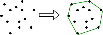
Fig 4: Convex hull

Input is an array of points specified by their x and y coordinates. The output is the convex hull of this set of points.

Examples:

Input: points [ ] = {(0, 0), (0, 4), (-4, 0), (5, 0),

(0, -6), (1, 0)};

Output: (-4, 0), (5, 0), (0, -6), (0, 4)

Application

In computational geometry, this is one of the oldest and most well-studied problems.

●      Motion planning for robots.

●      P. Is surrounded by the shortest perimeter fence.

●      P is encircled by the smallest area polygon.

●      P encloses a unique convex polygon whose vertices are points in P.

●      All N points are contained in the smallest convex set (i.e., intersection of all convex sets containing the N points).

Searching

The process of locating a desired object among a collection of items is referred to as searching. "target" is the name of the desired element. Any data structure, such as a list, array, linked-list, tree, or graph, can be used to search for objects.

In a collection of things, search refers to finding a desired element with defined qualities. The following are some of the most regularly used and straightforward search algorithms.

Linear search - The worst execution time for linear search is n, where n is the number of things searched.

Binary search - Binary search requires that objects be sorted, although it is substantially faster than linear search because its worst execution time is constant.

Interpolation search - Interpolation search requires that items be sorted, although it is substantially faster than linear search because its worst execution time is O(n), where n is the number of items.

Key takeaway

1. Any line segment connecting two points on the boundary of a polygon is convex if it stays within the polygon.
2. If you walk around the polygon's perimeter in a counterclockwise fashion, you will always turn left.
3. The process of locating a desired object among a collection of items is referred to as searching.

3.4 Greedy Methods with Examples Such as Optimal Reliability Allocation

A greedy algorithm is any algorithm that follows the problem-solving metaheuristic of making the locally optimal choice at each stage with the hope of finding the global optimum.

General Method:

Often, we are looking at optimization problems whose performance is exponential.

• For an optimization problem, we are given a set of constraints and an optimization function.

●      Solutions that satisfy the constraints are called feasible solutions.

●      A feasible solution for which the optimization function has the best possible value is called an optimal solution.

• Cheapest lunch possible: Works by getting the cheapest meat, fruit, vegetable, etc.

• By a greedy method we attempt to construct an optimal solution in stages.

●      At each stage we make a decision that appears to be the best (under some criterion) at the time.

●      A decision made at one stage is not changed in a later stage, so each decision should assure feasibility.

In general, greedy algorithms have five pillars:

1. A candidate set, from which a solution is created
2. A selection function, which chooses the best candidate to be added to the solution
3. A feasibility function, that is used to determine if a candidate can be used to contribute to a solution
4. An objective function, which assigns a value to a solution, or a partial solution, and
5. A solution function, which will indicate when we have discovered a complete solution

Greedy algorithms produce good solutions on some mathematical problems, but not on others. Most problems for which they work well have two properties:

Greedy choice property

We can make whatever choice seems best at the moment and then solve the sub problems that arise later. The choice made by a greedy algorithm may depend on choices made so far but not on future choices or all the solutions to the sub problem.

It iteratively makes one greedy choice after another, reducing each given problem into a smaller one. In other words, a greedy algorithm never reconsiders its choices. This is the main difference from dynamic programming, which is exhaustive and is guaranteed to find the solution.

After every stage, dynamic programming makes decisions based on all the decisions made in the previous stage, and may reconsider the previous stage's algorithmic path to solution.

Optimal substructure

"A problem exhibits optimal substructure if an optimal solution to the problem contains optimal solutions to the sub-problems."

Greedy method suggests that one can devise an algorithm that works in stages, considering one input at a time. At each stage, a decision is made regarding whether a particular input is an optimal solution. This is done by considering the inputs in an order determined by some selection procedure.

Algorithm Greedy (a, n)

//a [1: n] contains the n inputs.

{

Solution:= ø;  //Initialize the solution.

For i:=1 to n do

{

x:= Select(a);

If Feasible(solution, x) then

Solution: = Union(Solution, x);

}

Return solution;

}

The function Select selects an input from a[ ] and removes it. The selected input value is assigned to x. Feasible is a Boolean valued function that determines whether x can be included into the solution vector. Union combines x with the solution and updates the objective function.

Consider change making:

Given a coin system and an amount to make change for, we want minimal number of coins.

A greedy criterion could be, at each stage increase the total amount of change constructed as much as possible.

In other words, always pick the coin with the greatest value at every step.

A greedy solution is optimal for some change systems.

Machine scheduling:

Have a number of jobs to be done on a minimum number of machines. Each job has a start and end time. Order jobs by start time.

If an old machine becomes available by the start time of the task to be assigned, assign the task to this machine; if not assign it to a new machine.

This is an optimal solution.

Note that our Huffman tree algorithm is an example of a greedy algorithm:

Pick least weight trees to combine.

Key takeaway:

1. The greedy approach works well when applied to greedy-choice problems Real estate.
2. A set of local changes from a starting configuration will often find a globally-optimal solution.

3.5 Knapsack

● We are given n no. Of objects with weights Wi and profit Pi where I varies from 1 to n and also a knapsack with capacity M

● The problem is, we have to fill the bag with the help of n objects and the resulting profit has to be maximum.

● This problem is similar to the ordinary knapsack problem but we may not take a function of an object.

Example:

In this problem we find upper bound and lower bound for each node.

●  To calculate upper bound

Place first item in knapsack calculate remaining weight i.e., 15-2=13

Place next item in knapsack and remaining weight is 13-4=9

Place next item in knapsack and remaining weight is 9-6=3

Fraction is not allowed in calculation of upper bound in knapsack hence next item cannot be placed in the knapsack.

Profit=p1+p2+p3=10+10+12=32 i.e., Upper bound

●  To calculate lower bound

Fraction is allowed in calculation of lower bound in knapsack hence the next item can be placed in the knapsack.

Lower bound=10+10+12+(3/9*18) =32+6=38

Knapsack is a maximization problem but branch and bound can be applied on minimization problems.

Hence to convert maximization problem into minimization we have to take negative sign for upper bound and lower bound.

Therefore, upper bound (U)=-32

Lower bound(L)=-38

We choose the path which has minimized difference of upper bound and lower bound.

If the difference is equal then choose the path by comparing upper bound and discard node with maximize upper node.

Now calculate upper and lower bound for remaining nodes.

For node 2,

U=10+10+12=32 ≈ -32

L=10+10+12+(3/9*18) =32+6=38 ≈ -38

For node 3,

U=10+12=22

L=10+12+(5/9*18) =32 ≈ -32

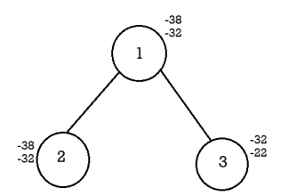
Calculate the difference of upper bound and lower bound for 2,3.

For node 2, U-L=-32+38=6

For node 3, U-L=-22+32=10

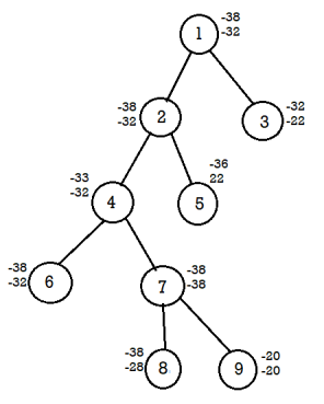
Select node 2 since it has a minimum difference value of 6.

Similarly continues the process,

Calculate difference of lower and upper bound of nodes 8 ,9.

For node 8, U-L=-38+38=0

For node 9, U-L=-20+20=0

Here the difference is the same hence compare the upper bound of node 8 and 9.

Discard the node with maximum upper bound.

Consider the path from 1→ 2→4→7→8

The solution for 0/1 knapsack problem is (1,1,0,1)

Maximum profit= ∑PiXi = 10*1+10*1+12*0+18*1=10+10+18=38

FIFO branch and bound solution

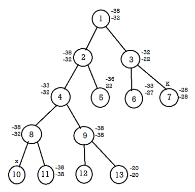
Let's assume the above example in this problem.

Initially node 1 is E node and the queue of live nodes are empty.

Here U=-32 hence node 2 and 3 are generated as children of node 1 and added to the queue. The value of the upper bound remains unchanged.

Now node 2 becomes E node and its children are added to the queue.

Next node 3 is expanded and its children are generated. Node 6 is also added to the queue. Node 7 is killed as L (7)>U.

Next node 4 is expanded. Continue the process until it gets the solution.

Key takeaways

1. This problem is similar to the ordinary knapsack problem but we may not take a function of an object.
2. We are given n no. Of objects with weights Wi and profit Pi where I vary from 1 to n and also a knapsack with capacity M

3.6 Minimum Spanning Trees – Prim’s and Kruskal’s Algorithms

●      If A is the set of edges selected so far, then A forms a tree.

●      The next edge (u, v) to be included in A is a minimum cost edge not in A with the property that A U {u, v} is also a tree.

●      Steps to solve the prim's algorithm:

Step 1: remove all loops and parallel edges

Step 2: chose any arbitrary node as root node

Step 3: check the outgoing edges and chose edge with the less value

Step 4: find the optimal solution by adding all the minimum cost of edges.

●      Example:

To find the MST, apply Prim's algorithm to the following graph.

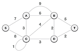
Solution:

Step1: Remove all loops and parallel edges

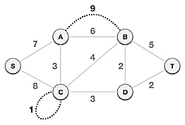
From the provided graph, remove any loops and parallel edges. If there are parallel edges, keep the one with the lowest cost and discard the others.

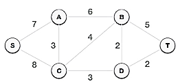
Step 2: Choose any arbitrary node as root node

In this scenario, the root node of Prim's spanning tree is S node. Because this node is picked at random, any node can be the root node. It's understandable to wonder why any video can be a root node. So, all the nodes of a graph are included in the spanning tree, and because it is connected, there must be at least one edge that connects it to the rest of the tree.

Step 3: Check outgoing edges and select the one with less cost

We can see that S, A and S, C are two edges with weights of 7 and 8, respectively, after selecting the root node S. The edge S, A is chosen since it is smaller than the other.

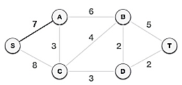
The tree S-7-A is now viewed as a single node, and all edges emanating from it are checked. We choose the one with the lowest price and put it on the tree.

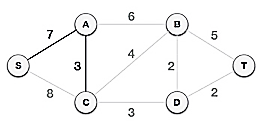
The S-7-A-3-C tree is generated after this phase. Now we'll treat it like a node again, and we'll double-check all of the edges. However, we will only select the lowest-cost advantage. In this scenario, the new edge is C-3-D, which costs less than the other edges' costs of 8, 6, 4, and so on.

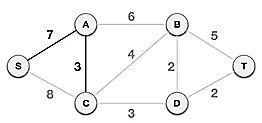
Following the addition of node D to the spanning tree, we now have two edges with the same cost, namely D-2-T and D-2-B. As a result, we can use any one. However, at the next step, edge 2 will again be the least expensive. As a result, we've drawn a spanning tree that includes both edges.

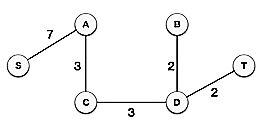
It's possible that the output spanning tree of two distinct algorithms for the same graph is the same.

Algorithm Prim(E, cost, n, t)

//E is the set of edges in G cost (1:n,1:n) is the adjacency matrix such at cost (i,j) is a +ve //real number or cost (i,j) is ∞ if no edge (i,j) exists. A minimum cost spanning tree is //computed and stored as a set of edges in the array T (1:n-1,1:2). (T(i,1), T(i,2) is an edge //in minimum cost spanning tree. The final cost is returned.

{

Let (k,l) to be an edge of minimum cost in E;

Mincost ß cost (k,l);

(T(1,1) T(1,2) )ß (k,l);

For  iß 1 to n do // initialing near

If  cost (i,L) < cost (I,k) then near (i) ß L ;

Else near (i) ß k ;

Near(k) ß near (l) ß 0;

For  i ß 2 to n-1 do

{

//find  n-2 additional edges for T

Let j be an index such that near (J) ¹ 0 and

Cost (J, near(J)) is minimum;

(T(i,1),T(i,2)) ß (j, NEAR (j));

Mincost ß mincost + cost (j,  near (j));

Near (j) ß 0;

For  k ß 1 to n do // update  near[]

If near (k) ¹ 0 and cost(k near (k)) > cost(k,j) then NEAR (k) ß j;

}

Return mincost;

}

Complexities:

A simple implementation using an adjacency matrix graph representation and searching an array of weights to find the minimum weight edge to add requires O(V2) running time.

Using a simple binary heap data structure and an adjacency list representation, Prim's algorithm can be shown to run in time O(E log V) where E is the number of edges and V is the number of vertices.

Using a more sophisticated Fibonacci heap, this can be brought down to O(E + V log V), which is asymptotically faster when the graph is dense enough that E is Ω(V).

Kruskal algorithm

Kruskal's Algorithm assembles the spanning tree by adding edges individually into a developing crossing tree. Kruskal's calculation follows a greedy approach as in every cycle it finds an edge which has least weight and add it to the developing traversing tree.

Calculation Steps:

Sort the chart edges concerning their loads.

Begin adding edges to the MST from the edge with the littlest load until the edge of the biggest weight.

Just add edges which doesn't frame a cycle, edges which interface just separated parts.

So now the inquiry is the means by which to check if vertices are associated or not?

This could be done using DFS which starts from the first vertex, then check if the second vertex is visited or not. But DFS will make time complexity large as it has an order of O(V+E) where V is the number of vertices, E is the number of edges. So, the best solution is "Disjoint Sets":

Disjoint sets will be setting whose crossing point is the unfilled set so it implies that they don't share any component practically speaking.

Think about after model:

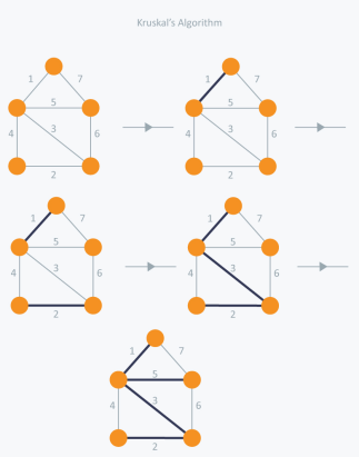
Figure 5

In Kruskal's algorithm, we pick the edge with the lowest weight for each iteration. So, first of all, we will start with the lowest weighted edge, i.e., the edges with weight 1. We would choose the second lowest weighted edge after that, i.e., the edge with weight 2. Notice that these two edges are absolutely disjointed. The third lowest weighted edge will now be the next edge, i.e., the edge with weight 3, which connects the two disjoint parts of the graph. Still, with weight 4, we are not able to choose the edge that will create a loop and we can't get any cycles.

But we are going to pick the fifth lowest weighted edge, i.e., the 5th weighted edge. Now the other two sides are trying to build loops, so we're going to forget them. In the end, we end up with a minimum spanning tree with total cost 11 (= 1 + 2 + 3 + 5).

Time Complexity:

In Kruskal’s algorithm, the most time-consuming operation is sorting because the total complexity of the Disjoint-Set operations will be O(ElogV), which is the overall Time Complexity of the algorithm.

Key takeaway

1. Prim's algorithm is a vertex algorithm based on
2. Prim's algorithm-needs priority queue for the nearest vertex position.\
3. Kruskal's Algorithm assembles the spanning tree by adding edges individually into a developing crossing tree.
4. Kruskal's calculation follows a greedy approach as in every cycle it finds an edge which has least weight and add it to the developing traversing tree.

3.7 Single Source Shortest Paths - Dijkstra’s and Bellman Ford Algorithms

Bellman-Ford Algorithm

Solves single shortest path problem in which edge weight may be negative but no negative cycle exists.

This algorithm works correctly when some of the edges of the directed graph G may have negative weight. When there are no cycles of negative weight, then we can find out the shortest path between source and destination.

It is slower than Dijkstra's Algorithm but more versatile, as it capable of handling some of the negative weight edges.

This algorithm detects the negative cycle in a graph and reports their existence.

Based on the "Principle of Relaxation" in which more accurate values gradually recovered an approximation to the proper distance by until eventually reaching the optimum solution.

Given a weighted directed graph G = (V, E) with source s and weight function w: E → R, the Bellman-Ford algorithm returns a Boolean value indicating whether or not there is a negative weight cycle that is attainable from the source. If there is such a cycle, the algorithm produces the shortest paths and their weights. The algorithm returns TRUE if and only if a graph contains no negative - weight cycles that are reachable from the source.

Recurrence Relation

Distk [u] = [min[distk-1 [u],min[ distk-1 [i]+cost [i,u]]] as i except u.

k → k is the source vertex

u → u is the destination vertex

i → no of edges to be scanned concerning a vertex.

BELLMAN -FORD (G, w, s)

1. INITIALIZE - SINGLE - SOURCE (G, s)

2. For i ← 1 to |V[G]| - 1

3. Do for each edge (u, v) ∈ E [G]

4. Do RELAX (u, v, w)

5. For each edge (u, v) ∈ E [G]

6. Do if d [v] > d [u] + w (u, v)

7. Then return FALSE.

8. Return TRUE.

Example: Here first we list all the edges and their weights.

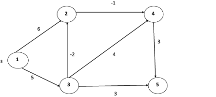
Solution:

Distk [u] = [min[distk-1 [u],min[distk-1 [i]+cost [i,u]]] as i ≠ u.

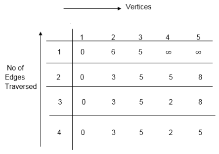
Dist2 [2]=min[dist1 [2],min[dist1 [1]+cost[1,2],dist1 [3]+cost[3,2],dist1 [4]+cost[4,2],dist1 [5]+cost[5,2]]]

Min = [6, 0 + 6, 5 + (-2), ∞ + ∞ , ∞ +∞] = 3

Dist2 [3]=min[dist1 [3],min[dist1 [1]+cost[1,3],dist1 [2]+cost[2,3],dist1 [4]+cost[4,3],dist1 [5]+cost[5,3]]]

Min = [5, 0 +∞, 6 +∞, ∞ + ∞ , ∞ + ∞] = 5

Dist2 [4]=min[dist1 [4],min[dist1 [1]+cost[1,4],dist1 [2]+cost[2,4],dist1 [3]+cost[3,4],dist1 [5]+cost[5,4]]]

Min = [∞, 0 +∞, 6 + (-1), 5 + 4, ∞ +∞] = 5

Dist2 [5]=min[dist1 [5],min[dist1 [1]+cost[1,5],dist1 [2]+cost[2,5],dist1 [3]+cost[3,5],dist1 [4]+cost[4,5]]]

Min = [∞, 0 + ∞,6 + ∞,5 + 3, ∞ + 3] = 8

Dist3 [2]=min[dist2 [2],min[dist2 [1]+cost[1,2],dist2 [3]+cost[3,2],dist2 [4]+cost[4,2],dist2 [5]+cost[5,2]]]

Min = [3, 0 + 6, 5 + (-2), 5 + ∞ , 8 + ∞ ] = 3

Dist3 [3]=min[dist2 [3],min[dist2 [1]+cost[1,3],dist2 [2]+cost[2,3],dist2 [4]+cost[4,3],dist2 [5]+cost[5,3]]]

Min = [5, 0 + ∞, 3 + ∞, 5 + ∞,8 + ∞ ] = 5

Dist3 [4]=min[dist2 [4],min[dist2 [1]+cost[1,4],dist2 [2]+cost[2,4],dist2 [3]+cost[3,4],dist2 [5]+cost[5,4]]]

Min = [5, 0 + ∞, 3 + (-1), 5 + 4, 8 + ∞ ] = 2

Dist3 [5]=min[dist2 [5],min[dist2 [1]+cost[1,5],dist2 [2]+cost[2,5],dist2 [3]+cost[3,5],dist2 [4]+cost[4,5]]]

Min = [8, 0 + ∞, 3 + ∞, 5 + 3, 5 + 3] = 8

Dist4 [2]=min[dist3 [2],min[dist3 [1]+cost[1,2],dist3 [3]+cost[3,2],dist3 [4]+cost[4,2],dist3 [5]+cost[5,2]]]

Min = [3, 0 + 6, 5 + (-2), 2 + ∞, 8 + ∞ ] =3

Dist4 [3]=min[dist3 [3],min[dist3 [1]+cost[1,3],dist3 [2]+cost[2,3],dist3 [4]+cost[4,3],dist3 [5]+cost[5,3]]]

Min = 5, 0 + ∞, 3 + ∞, 2 + ∞, 8 + ∞ ] =5

Dist4 [4]=min[dist3 [4],min[dist3 [1]+cost[1,4],dist3 [2]+cost[2,4],dist3 [3]+cost[3,4],dist3 [5]+cost[5,4]]]

Min = [2, 0 + ∞, 3 + (-1), 5 + 4, 8 + ∞ ] = 2

Dist4 [5]=min[dist3 [5],min[dist3 [1]+cost[1,5],dist3 [2]+cost[2,5],dist3 [3]+cost[3,5],dist3 [5]+cost[4,5]]]

Min = [8, 0 +∞, 3 + ∞, 8, 5] = 5

Dijkstra's Algorithm

It is a greedy algorithm that solves the single-source shortest path problem for a directed graph G = (V, E) with nonnegative edge weights, i.e., w (u, v) ≥ 0 for each edge (u, v) ∈ E.

Dijkstra's Algorithm maintains a set S of vertices whose final shortest - path weights from the source s have already been determined. That's for all vertices v ∈ S; we have d [v] = δ (s, v). The algorithm repeatedly selects the vertex u ∈ V - S with the minimum shortest - path estimate, insert u into S and relaxes all edges leaving u.

Because it always chooses the "lightest" or "closest" vertex in V - S to insert into set S, it is called as the greedy strategy.

Dijkstra's Algorithm (G, w, s)

1. INITIALIZE - SINGLE - SOURCE (G, s)

2. S←∅

3. Q←V [G]

4. While Q ≠ ∅

5. Do u ← EXTRACT - MIN (Q)

6. S ← S ∪ {u}

7. For each vertex v ∈ Adj [u]

8. Do RELAX (u, v, w)

Analysis: The running time of Dijkstra's algorithm on a graph with edges E and vertices V can be expressed as a function of |E| and |V| using the Big - O notation. The simplest implementation of the Dijkstra's algorithm stores vertices of set Q in an ordinary linked list or array, and operation Extract - Min (Q) is simply a linear search through all vertices in Q. In this case, the running time is O (|V2 |+|E|=O(V2 ).

Example:

Solution:

Step1: Q =[s, t, x, y, z]

We scanned vertices one by one and find out its adjacent. Calculate the distance of each adjacent to the source vertices.

We make a stack, which contains those vertices which are selected after computation of shortest distance.

Firstly, we take's' in stack M (which is a source)

1. M = [S] Q = [t, x, y, z] 

Step 2: Now find the adjacent of s that are t and y.

1. Adj [s] → t, y [Here s is u and t and y are v] 

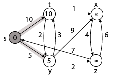
Case - (i) s → t

d [v] > d [u] + w [u, v]

d [t] > d [s] + w [s, t]

∞ > 0 + 10                [false condition]

Then       d [t] ← 10

π [t] ← 5

Adj [s] ← t, y

Case - (ii) s→ y

d [v] > d [u] + w [u, v]

d [y] > d [s] + w [s, y]

∞ > 0 + 5                [false condition]

∞ > 5

Then       d [y] ← 5

π [y] ← 5

By comparing case (i) and case (ii)

Adj [s] → t = 10, y = 5

y is shortest

y is assigned in 5 = [s, y]

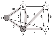
Step 3: Now find the adjacent of y that is t, x, z.

1. Adj [y] → t, x, z   [Here y is u and t, x, z are v] 

Case - (i) y →t

d [v] > d [u] + w [u, v]

d [t] > d [y] + w [y, t]

10 > 5 + 3

10 > 8

Then     d [t] ← 8

π [t] ← y

Case - (ii) y → x

d [v] > d [u] + w [u, v]

d [x] > d [y] + w [y, x]

∞ > 5 + 9

∞ > 14

Then      d [x] ← 14

π [x] ← 14

Case - (iii) y → z

d [v] > d [u] + w [u, v]

d [z] > d [y] + w [y, z]

∞ > 5 + 2

∞ > 7

Then      d [z] ← 7

π [z] ← y

By comparing case (i), case (ii) and case (iii)

Adj [y] → x = 14, t = 8, z =7

z is shortest

z is assigned in 7 = [s, z]

Step - 4 Now we will find adj [z] that are s, x

1. Adj [z] → [x, s]  [Here z is u and s and x are v] 

Case - (i) z → x

d [v] > d [u] + w [u, v]

d [x] > d [z] + w [z, x]

14 > 7 + 6

14 > 13

Then       d [x] ← 13

π [x] ← z

Case - (ii) z → s

d [v] > d [u] + w [u, v]

d [s] > d [z] + w [z, s]

0 > 7 + 7

0 > 14

∴ This condition does not satisfy so it will be discarded.

Now we have x = 13.

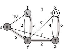
Step 5: Now we will find Adj [t]

Adj [t] → [x, y] [Here t is u and x and y are v]

Case - (i) t → x

d [v] > d [u] + w [u, v]

d [x] > d [t] + w [t, x]

13 > 8 + 1

13 > 9

Then       d [x] ← 9

π [x] ← t

Case - (ii) t → y

d [v] > d [u] + w [u, v]

d [y] > d [t] + w [t, y]

5 > 10

∴ This condition does not satisfy so it will be discarded.

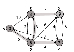
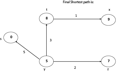
Thus, we get all shortest path vertex as

Weight from s to y is 5

Weight from s to z is 7

Weight from s to t is 8

Weight from s to x is 9

These are the shortest distance from the source's' in the given graph.

Disadvantage of Dijkstra's Algorithm:

1. It does a blind search, so wastes a lot of time while processing.
2. It can't handle negative edges.
3. It leads to the acyclic graph and most often cannot obtain the right shortest path.
4. We need to keep track of vertices that have been visited.

In Dijkstra’s algorithm, two sets are maintained, one set contains list of vertices already included in SPT (Shortest Path Tree), other set contains vertices not yet included. With adjacency list representation, all vertices of a graph can be traversed in O(V+E) time using BFS.

The idea is to traverse all vertices of graph using BFS and use a Min Heap to store the vertices not yet included in SPT (or the vertices for which shortest distance is not finalized yet).  Min Heap is used as a priority queue to get the minimum distance vertex from set of not yet included vertices.  Time complexity of operations like extract-min and decrease-key value is O(LogV) for Min Heap.

Following are the detailed steps.

1) Create a Min Heap of size V where V is the number of vertices in the given graph. Every node of min heap contains vertex number and distance value of the vertex.

2) Initialize Min Heap with source vertex as root (the distance value assigned to source vertex is 0). The distance value assigned to all other vertices is INF (infinite).

3) While Min Heap is not empty, do following

a) Extract the vertex with minimum distance value node from Min Heap. Let the extracted vertex be u.

b) For every adjacent vertex v of u, check if v is in Min Heap. If v is in Min Heap and distance value is more than weight of u-v plus distance value of u, then update the distance value of v.

Let us understand with the following example. Let the given source vertex be 0

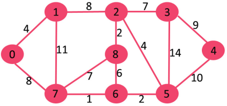
Initially, distance value of source vertex is 0 and INF (infinite) for all other vertices. So, source vertex is extracted from Min Heap and distance values of vertices adjacent to 0 (1 and 7) are updated. Min Heap contains all vertices except vertex 0.

The vertices in green color are the vertices for which minimum distances are finalized and are not in Min Heap

Since distance value of vertex 1 is minimum among all nodes in Min Heap, it is extracted from Min Heap and distance values of vertices adjacent to 1 are updated (distance is updated if a vertex is in Min Heap and distance through 1 is shorter than the previous distance). Min Heap contains all vertices except vertex 0 and 1.

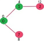
Pick the vertex with minimum distance value from min heap. Vertex 7 is picked. So, min heap now contains all vertices except 0, 1 and 7. Update the distance values of adjacent vertices of 7. The distance value of vertex 6 and 8 becomes finite (15 and 9 respectively).

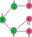
Pick the vertex with minimum distance from min heap. Vertex 6 is picked. So, min heap now contains all vertices except 0, 1, 7 and 6. Update the distance values of adjacent vertices of 6. The distance value of vertex 5 and 8 are updated.

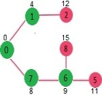
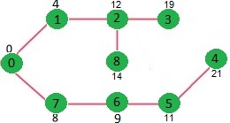
Above steps are repeated till min heap doesn’t become empty. Finally, we get the following shortest path tree.

// A C/C++ program for Dijkstra's single source shortest path algorithm.

// The program is for adjacency matrix representation of the graph

#include <limits.h>

#include <stdio.h>

#include  <stdbool.h>

// Number of vertices in the graph

#define V 9

// A utility function to find the vertex with minimum distance value, from

// the set of vertices not yet included in shortest path tree

Int minDistance(int dist[], bool sptSet[])

{

// Initialize min value

Int min = INT_MAX, min_index;

For (int v = 0; v < V; v++)

If (sptSet[v] == false && dist[v] <= min)

Min = dist[v], min_index = v;

Return min_index;

}

// A utility function to print the constructed distance array

Void printSolution(int dist[])

{

Printf("Vertex \t\t Distance from Source\n");

For (int i = 0; i < V; i++)

Printf("%d \t\t %d\n", i, dist[i]);

}

// Function that implements Dijkstra's single source shortest path algorithm

// for a graph represented using adjacency matrix representation

Void dijkstra(int graph[V][V], int src)

{

Int dist[V]; // The output array.  dist[i] will hold the shortest

// distance from src to i

Bool sptSet[V]; // sptSet[i] will be true if vertex i is included in shortest

// path tree or shortest distance from src to i is finalized

// Initialize all distances as INFINITE and stpSet[] as false

For (int i = 0; i < V; i++)

Dist[i] = INT_MAX, sptSet[i] = false;

// Distance of source vertex from itself is always 0

Dist[src] = 0;

// Find shortest path for all vertices

For (int count = 0; count < V - 1; count++) {

// Pick the minimum distance vertex from the set of vertices not

// yet processed. u is always equal to src in the first iteration.

Int u = minDistance(dist, sptSet);

// Mark the picked vertex as processed

SptSet[u] = true;

// Update dist value of the adjacent vertices of the picked vertex.

For (int v = 0; v < V; v++)

// Update dist[v] only if is not in sptSet, there is an edge from

// u to v, and total weight of path from src to  v through u is

// smaller than current value of dist[v]

If (!sptSet[v] && graph[u][v] && dist[u] != INT_MAX

&& dist[u] + graph[u][v] < dist[v])

Dist[v] = dist[u] + graph[u][v];

}

// print the constructed distance array

PrintSolution(dist);

}

// driver program to test above function

Int main()

{

/* Let us create the example graph discussed above */

Int graph[V][V] = {{0, 4, 0, 0, 0, 0, 0, 8, 0},

{ 4, 0, 8, 0, 0, 0, 0, 11, 0 },

{ 0, 8, 0, 7, 0, 4, 0, 0, 2 },

{ 0, 0, 7, 0, 9, 14, 0, 0, 0 },

{ 0, 0, 0, 9, 0, 10, 0, 0, 0 },

{ 0, 0, 4, 14, 10, 0, 2, 0, 0 },

{ 0, 0, 0, 0, 0, 2, 0, 1, 6 },

{ 8, 11, 0, 0, 0, 0, 1, 0, 7 },

{ 0, 0, 2, 0, 0, 0, 6, 7, 0 } };

Dijkstra(graph, 0);

Return 0;

}

Output:

Vertex   Distance from Source

0                0

1                4

2                12

3                19

4                21

5                11

6                9

7                8

8                14

Time Complexity: The time complexity of the above code/algorithm looks O(V^2) as there are two nested while loops. If we take a closer look, we can observe that the statements in inner loop are executed O(V+E) times (similar to BFS). The inner loop has decreaseKey() operation which takes O(LogV) time. So overall time complexity is O(E+V)*O(LogV) which is O((E+V)*LogV) = O(ELogV)

Note that the above code uses Binary Heap for Priority Queue implementation. Time complexity can be reduced to O(E + VLogV) using Fibonacci Heap. The reason is, Fibonacci Heap takes O(1) time for decrease-key operation while Binary Heap takes O(Logn) time.

Key takeaway

1. The code calculates shortest distance, but doesn’t calculate the path information. We can create a parent array, update the parent array when distance is updated (like prim’s implementation) and use it show the shortest path from source to different vertices.
2. The code is for undirected graphs; the same dijkstra function can be used for directed graphs also.
3. The code finds shortest distances from source to all vertices. If we are interested only in shortest distance from source to a single target, we can break the for loop when the picked minimum distance vertex is equal to target (Step 3.a of algorithm).
4. Dijkstra’s algorithm doesn’t work for graphs with negative weight edges. For graphs with negative weight edges, Bellman–Ford algorithm can be used.

References:

1. Thomas H. Coreman, Charles E. Leiserson and Ronald L. Rivest, “Introduction to Algorithms”, Printice Hall of India.

2. E. Horowitz & S Sahni, "Fundamentals of Computer Algorithms",

3. Aho, Hopcraft, Ullman, “The Design and Analysis of Computer Algorithms” Pearson Education, 2008.

4. LEE "Design & Analysis of Algorithms (POD)", McGraw Hill

5. Richard E.Neapolitan "Foundations of Algorithms" Jones & Bartlett Learning