Unit – 4

Dynamic Programming

4.1 Dynamic Programming with Examples Such as Knapsack

The most powerful design tool for solving optimization problems is Dynamic Programming.

The Divide & Conquer algorithm divides the problem into separate subproblems, which are then solved recursively before being combined to solve the original problems.

When the subproblems are not independent, such as when they share the same subproblems, Dynamic Programming is utilized. Because it solves the same subproblem numerous times, divide and conquer may do more work than is necessary in this case.

Dynamic Programming solves each subproblem just once and saves the result in a database so it can be retrieved again if necessary.

Dynamic Programming is a Bottom-up approach in which we solve all potential little problems before combining them to address larger problems.

Dynamic Programming is an algorithm design paradigm in which an optimization problem is handled using a combination of sub-problem solutions and the "principle of optimality."

Characteristics

When an issue has the following characteristics, Dynamic Programming can help:

Optimal Substructure: A problem has optimum substructure if an ideal solution comprises optimal sub solutions.

Overlapping subproblems: A problem has overlapping subproblems when a recursive algorithm visits the same subproblems again.

We can recursively define an optimal solution if a problem has optimal substructure. When a problem involves overlapping subproblems, a recursive implementation can be improved by computing each subproblem just once.

There is no basis for constructing a recursive method to identify the optimal solutions if the problem does not have optimal substructure. We have nothing to gain from using dynamic programming if a problem does not have overlapping subproblems.

Dynamic programming can be substantially more efficient than recursion if the space of subproblems is large enough (i.e. polynomial in the size of the input).

Example - Knapsack

Given a knapsack capacity c ∈ N and n objects A = {a0, . . . , an−1}, each having a nonnegative value v(ai) ∈ {x ∈ R : x ≥ 0} and a weight w(ai) ∈ N, the 0/1 knapsack problem (KS01) asks to pack the knapsack with a subset of objects from A, such that the sum of the weight of the chosen objects does not exceed the capacity c, and such that the sum of the values of the chosen objects is maximal.

Let xi denote the binary decision variable of whether to include (i.e. xi = 1) object ai, or not (i.e. xi = 0). For brevity, we write vi for v(ai) and wi for w(ai). KS01 can also be formally stated as an integer LP

Problem:

Max  z =  

s.t.      ≤ c

Xi ∈ {0, 1} ∀i ∈ {0, . . . , n − 1}.

The KS01 problem can be interpreted as a multistage decision problem in a straightforward manner. For each object ai, a decision xi has to be made whether to include ai, or not. Let the stage number i denote the index of the object currently under consideration and let w denote the space currently available in the knapsack.

The DP functional equation is

f(i,w) = 0     if i = −1 and 0 ≤ w ≤ c

−∞      if i = −1 and w < 0

Max {xivi + f(i − 1, w − xiwi)} if i ≥ 0

Xi∈{0,1}

The goal is to compute f(n−1, c). The above DP functional equation can be slightly improved by introducing a decision set

D = D(i,w) = _{0} if wi > w

{0, 1} if wi ≤ w.

That disallows infeasible decisions instead of punishing illegal states with a −∞ assignment. Replacing the static decision set {0, 1} used in (2.24) we get

f(i,w) = 0      if i = −1 and 0 ≤ w ≤ c

Max {xivi + f(i − 1, w − xiwi)}  if i ≥ 0

Xi∈D

For instance, let c = 22, n = 3, A = (a0, a1, a2), (v0, v1, v2) = (25, 24, 15), and (w0, w1, w2) = (18, 15, 10). Then it is optimal to pick only object a0, in the final (i = 0) stage, and the optimal value of the knapsack is f(2, 22) = 25.

The integer knapsack problem, a variation of KS01 that allows integral decision variables xi, can be reduced to KS01, and vice versa.

●      0/1 knapsack problem is used to find the maximum profit from the items selected.

●      0/1 knapsack problem means we pick the item or not picking the item ie. We can't split the item.

●      Item having the weight and the cost.

●      Assume we are having many items then which item will give us more profit than we have to check first.

●      First sort the value to weight in non-increasing order and then pick the item.

Here I is row and j is column

If (j<wt[i])

T[i][j]=T[i-1][j]

Else

{

T[i][j]=max{val[i]+T[i-1][j-wt[i]]

Or

{T[i-1][j]

Here total weight =7

Key takeaway

1. The most powerful design tool for solving optimization problems is Dynamic Programming.
2. Dynamic Programming solves each subproblem just once and saves the result in a database so it can be retrieved again if necessary.
3. 0/1 knapsack problem is used to find the maximum profit from the items selected.
4. 0/1 knapsack problem means we pick the item or not picking the item ie. We can't split the item.

4.2 All Pair Shortest Paths – Warshall’s and Floyd’s Algorithms

Floyd-Warshall Algorithm

Let the vertices of G be V = {1, 2........n} and consider a subset {1, 2........k} of vertices for some k. For any pair of vertices i, j ∈ V, considered all paths from i to j whose intermediate vertices are all drawn from {1, 2.......k}, and let p be a minimum weight path from amongst them. The Floyd-Warshall algorithm exploits a link between path p and shortest paths from i to j with all intermediate vertices in the set {1, 2.......k-1}. The link depends on whether or not k is an intermediate vertex of path p.

If k is not an intermediate vertex of path p, then all intermediate vertices of path p are in the set {1, 2........k-1}. Thus, the shortest path from vertex i to vertex j with all intermediate vertices in the set {1, 2.......k-1} is also the shortest path i to j with all intermediate vertices in the set {1, 2.......k}.

If k is an intermediate vertex of path p, then we break p down into i → k → j.

Let dij(k) be the weight of the shortest path from vertex i to vertex j with all intermediate vertices in the set {1, 2.......k}.

A recursive definition is given by

FLOYD - WARSHALL (W)

1. n ← rows [W].

2. D0 ← W

3. For k ← 1 to n

4. Do for i ← 1 to n    

5. Do for j ← 1 to n    

6. Do dij(k) ← min (dij(k-1),dik(k-1)+dkj(k-1) )

7. Return D(n)     

The strategy adopted by the Floyd-Warshall algorithm is Dynamic Programming. The running time of the Floyd-Warshall algorithm is determined by the triply nested for loops of lines 3-6. Each execution of line 6 takes O (1) time. The algorithm thus runs in time θ(n3 ).

Example: Apply Floyd-Warshall algorithm for constructing the shortest path. Show that matrices D(k) and π(k) computed by the Floyd-Warshall algorithm for the graph.

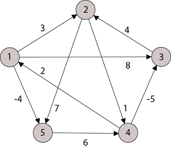
Solution:

Step (i) When k = 0

	3	8		-4		1	1	NIL	1
	0		1	7	Nil	Nil	Nil	2	2
	4	0	-5		Nil	3	Nil	3	Nil
2			0		4	Nil	Nil	Nil	Nil
			6	0	Nil	Nil	Nil	5	Nil

Step (ii) When k =1

	3	8		-4		1	1	NIL	1
	0		1	7	Nil	Nil	Nil	2	2
	4	0	-5		Nil	3	Nil	3	Nil
2	5	10	0	-2	4	1	1	Nil	1
			6	0	Nil	Nil	Nil	5	Nil

Step (iii) When k = 2

	3	8	4	-4		1	1	2	1
	0		1	7	Nil	Nil	Nil	2	2
	4	0	-5	11	Nil	3	Nil	3	2
2	5	10	0	-2	4	1	1	Nil	1
			6	0	Nil	Nil	Nil	5	Nil

Step (iv) When k = 3

Step (v) When k = 4

	3	8	4	-4		1	1	3	1
3	0	11	1	-1	4	Nil	4	2	2
-3	4	0	-5	-7	4	4	Nil	3	4
2	5	10	0	-2	4	1	1	Nil	1
8	11	16	6	0	4	4	4	5	Nil

Step (vi) When k = 5

	3	8	3	-4		1	1	5	1
3	0	11	1	-1	4	Nil	4	2	4
-3	0	0	-5	-7	4	4	Nil	3	4
2	5	10	0	-2	4	1	1	Nil	1
8	11	16	6	0	4	4	4	5	Nil

TRANSITIVE- CLOSURE (G)

1. n ← |V[G]|

2. For i ← 1 to n

3. Do for j ← 1 to n

4. Do if i = j or (i, j) ∈ E [G]

5. The ← 1

6. Else ← 0

7. For k ← 1 to n

8. Do for i ← 1 to n

9. Do for j ← 1 to n

10. Dod ij(k) ←  

11. Return T(n).

Key takeaway

1. The Floyd-Warshall algorithm exploits a link between path p and shortest paths from i to j with all intermediate vertices in the set {1, 2.......k-1}.
2. The link depends on whether or not k is an intermediate vertex of path p.
3. The strategy adopted by the Floyd-Warshall algorithm is Dynamic Programming.

4.3 Resource Allocation Problem

Resource allocation is the process of allocating available resources in a cost-effective manner. Resource allocation in project management refers to the planning of activities and the resources required by these activities while taking into account both resource availability and project time.

Strategic Planning and Resource Leveling are the two aspects of resource allocation.

1. Strategic planning –

Resource allocation in strategic planning refers to a strategy for utilizing available resources, such as human resources, in the short term to achieve long-term objectives. The process of allocating resources among several projects or corporate divisions is known as resource allocation. The strategic planning has 2 parts.

●      There is the basic allocation decision.

●      There is the contingency mechanism.

The basic allocation decision is to decide which plan items to support and at what level, as well as which to leave unfilled; resources are allocated to certain items but not to others.

There may be a contingency mechanism in place, such as a priority rating of items not included in the plan, indicating which items will be sacrificed in order to lower overall funding.

2.     Resource leveling –

The basic goal is to moderate resource demand by relocating slack jobs outside of high demand periods. Some of the approaches effectively mimic what a human scheduler would do if he had the time, procedures created specifically for the machine. They, of course, rely on the speed and capability of electronic compilers to succeed.

Approach for resource allocation:

There are number of approaches to solve resource allocation problems:

●      Manual Approach

●      Algorithmic Approach

●      Combination of both

The algorithmic technique allocates resources by employing a computer program that is defined for a certain area and distributes them automatically and dynamically to the user. This technology is often used in electronic devices that are specialized for routing and communication. For example, in wireless communication, channel allocation may be determined by the base transceiver using an appropriate algorithm.

Key takeaway

1. Resource allocation is the process of allocating available resources in a cost-effective manner.
2. Resource allocation in project management refers to the planning of activities and the resources required by these activities while taking into account both resource availability and project time.

4.4 Backtracking

It is a general algorithmic technique

● Backtracking algorithm is used to solve a problem recursively to get a solution incrementally.

● It is used to solve problems when the sequence of objects is chosen from a specified set so that the sequence can satisfy some criteria.

● Backtracking is the systematic method which helps to try out a sequence of decisions until you find out that solution.

● It starts with one smaller piece at a time, if its solution get fails to satisfy the constraint then it can be removed at any point of time.

● It searches for any possible combination in order to solve a computational problem.

Fig: A - backtracking

However, we usually design our trees from the top down, with the root at the bottom.

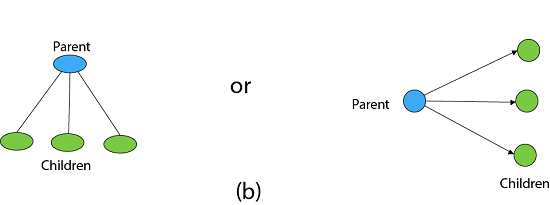
Fig: Backtracking

Nodes are the building blocks of a tree.

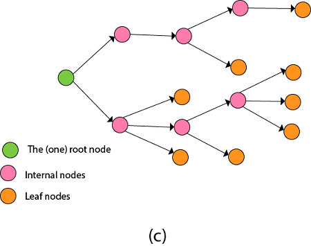
Fig: Backtracking

Backtracking is similar to searching a tree for a certain "target" leaf node.

Backtracking is straightforward: we "examine" each node as follows:

To "explore" node N:

1. If N is a goal node, return "success"

2. If N is a leaf node, return "failure"

3. For each child C of N,

Explore C

If C was successful, return "success"

4. Return "failure"

● Two constraints:

1. Implicit constraint
2. Explicit constraint

The backtracking algorithm finds the solution by scanning the solution space for the given problem in a systematic manner. With any bounding function, backtracking is a depth-first search. All backtracking solutions are required to fulfill a complex set of restrictions. Constraints might be stated explicitly or implicitly.

The Explicit Constraint is enforced, which limits each vector element's selection to the supplied set.

Implicit Constraint is ruled, which determines which each of the tuples in the solution space actually satisfy the criterion function.

● Application:

1. N-queen problem
2. Sum of subset
3. Graph coloring
4. Hamilton problems

Key takeaway

1. Backtracking algorithm is used to solve a problem recursively to get a solution incrementally.
2. It is used to solve problems when the sequence of objects is chosen from a specified set so that the sequence can satisfy some criteria.

4.5 Branch and Bound with Examples Such as Travelling Salesman Problem

Branch and bind is a method of designing algorithms that is commonly used to solve combinatorial optimization problems. In the worst-case scenario, these issues have exponential time complexity and may necessitate examining all potential permutations. These issues are solved rather rapidly using the Branch and Bound Algorithm approach.

Traveling-salesman Problem

In the traveling salesman Problem, a salesman must visits n cities. We can say that a salesman wishes to make a tour or Hamiltonian cycle, visiting each city exactly once and finishing at the city he starts from. There is a non-negative cost c (i, j) to travel from the city i to city j. The goal is to find a tour of minimum cost. We assume that every two cities are connected. Such problems are called the Traveling-salesman problem (TSP).

We can model the cities as a complete graph of n vertices, where each vertex represents a city.

It can be shown that TSP is NPC.

If we assume the cost function c satisfies the triangle inequality, then we can use the following approximate algorithm.

Triangle inequality

Let u, v, w be any three vertices, we have

One important observation to develop an approximate solution is if we remove an edge from H*, the tour becomes a spanning tree.

1. Approx-TSP (G= (V, E))  
2. { 
3. 1. Compute a MST T of G; 
4. 2. Select any vertex r is the root of the tree; 
5. 3. Let L be the list of vertices visited in a preorder tree walk of T; 
6. 4. Return the Hamiltonian cycle H that visits the vertices in the order L; 
7. } 

Traveling-salesman Problem

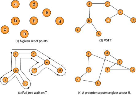
Fig - Traveling-salesman Problem

Intuitively, Approx-TSP first makes a full walk of MST T, which visits each edge exactly two times. To create a Hamiltonian cycle from the full walk, it bypasses some vertices (which corresponds to making a shortcut)

Key takeaway

1. Branch and bind is a method of designing algorithms that is commonly used to solve combinatorial optimization problems.
2. In the worst-case scenario, these issues have exponential time complexity and may necessitate examining all potential permutations.

4.6 Graph Coloring

Graph coloring is a basic method of labeling graph components including vertices, edges, and regions while adhering to certain criteria. No two nearby vertices, adjacent edges, or adjacent areas in a graph are colored with the same set of colors. This value is referred to as the chromatic number, and the graph is referred to as a properly colored graph.

Colors, sequence of coloring, method of assigning color, and other constraints are imposed on the graph during graph coloring. A vertex or a specific region is given a color. As a result, vertices or areas with the same color create separate sets.

Vertex coloring

The assigning of colors to the vertices of a graph ‘G' in such a way that no two adjacent vertices have the same color is known as ertex coloring. Simply put, an edge's vertices should not be the same color.

Chromatic Number

The chromatic number of G, indicated as X, is the lowest number of colors necessary for vertex coloring of graph ‘G.' (G).

If and only if 'G' is a null graph, (G) = 1. If the graph 'G' isn't a null graph, then χ(G) ≥ 2.

Example

Region coloring

The assignment of colors to the regions of a planar graph in such a way that no two neighboring regions have the same color is known as region coloring. If two regions share a common edge, they are said to be neighboring.

Example

Take a look at the graph below. Because there is a common edge ‘be' between the regions ‘aeb' and ‘befc,' they are adjacent.

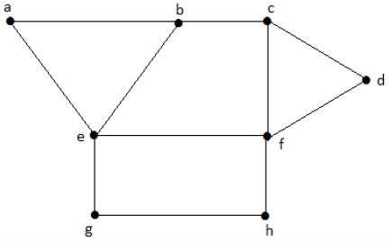
Similarly, the other regions are colored according to their proximity. The following colors are used to color this graph:

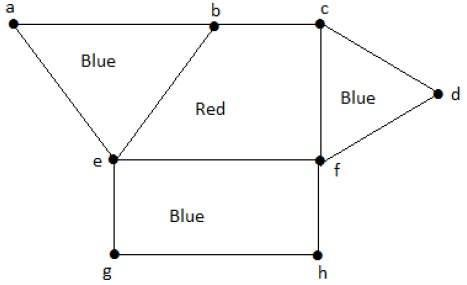
Application

One of the most significant notions in graph theory is graph coloring. It is utilized in a variety of real-time computer science applications, including

●      Clustering

●      Data mining

●      Image capturing

●      Image segmentation

●      Networking

●      Resource allocation

●      Processes scheduling

Key takeaway

1. Graph coloring is a basic method of labeling graph components including vertices, edges, and regions while adhering to certain criteria.
2. No two nearby vertices, adjacent edges, or adjacent areas in a graph are colored with the same set of colors.
3. This value is referred to as the chromatic number, and the graph is referred to as a properly colored graph.

4.7 n-Queen Problem

● Let chess board having N*N cells.

● We need to place N queens in such a way that no queen is attacked by any other queen.

● The queen can attack horizontally, vertically and diagonally.So initially, we are having N*N unattacked cells where we can place the N queens.

Step 1: Place the first queen at a cell (i,j). Hence the unattacked cell is reduced and the number of queens to be placed is N−1.

Step 2: Place the second queen on an unattacked cell that will reduce the no. Of unattacked cells and no. Of queen to be placed become N-2.

The process continues until it satisfies the following condition.

The no. Of unattacked cell become 0

The no of queens to be placed is not 0.

Step 3: As it satisfies the first condition given above then it’s over, we got a final solution.

But if the unattacked cells become 0, then we need to backtrack and remove the last placed queen from its current place and place it in another cell.

This process will be done recursively.

Example:

8-Queen problem

●  The eight-queen problem is the problem of placing eight queens on an 8×8 chessboard such that none of them attack one another.

●  The eight-queen puzzle has 92 distinct solutions.

●  If a solution that differs only by symmetry operation of the board are counted as one puzzle has 12 unique solutions.

Formulation of problem:

● States: any arrangement of 8 queens on board

● Initial state: 0 queens on the board

● Successor function: add a queen on any square

● Goal state: unattacked 8 queens on the board

Steps to be perform:

1. Place the first queen in the left upper corner of the table
2. Save the attacked position
3. Move to the next queen which can only be placed on next line
4. Search for a valid position. (unattacked position) If there is one go to step 8.
5. There is not a valid position for a queen then delete it.
6. Move to the previous queen
7. Got to step 4
8. Place it to the first valid position
9. Save the attacked positions
10. If the queen processed is the last stop otherwise go to step 3.

Algorithm:     

PutQueen(row)

{

For every position col on the same row

If the position col is available

Place the next queen in position col

If(row<8)

PutQueen(row+1)

Else success

Remove the queen from positioncol

}

4.8 Hamiltonian Cycles and Sum of Subsets

We must use the Backtracking technique to identify the Hamiltonian Circuit given a graph G = (V, E). We begin our search at any random vertex, such as 'a.' The root of our implicit tree is this vertex 'a.' The first intermediate vertex of the Hamiltonian Cycle to be constructed is the first element of our partial solution. By alphabetical order, the next nearby vertex is chosen.

A dead end is reached when any arbitrary vertices forms a cycle with any vertex other than vertex 'a' at any point. In this situation, we backtrack one step and restart the search by selecting a new vertex and backtracking the partial element; the answer must be removed. If a Hamiltonian Cycle is found, the backtracking search is successful.

Example - Consider the graph G = (V, E) in fig. We must use the Backtracking method to find a Hamiltonian circuit.

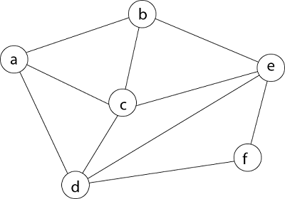
To begin, we'll start with vertex 'a,' which will serve as the root of our implicit tree.

Following that, we select the vertex 'b' adjacent to 'a' because it is the first in lexicographical order (b, c, d).

Then, next to 'b,' we select 'c.'

Next, we choose the letter 'd,' which is adjacent to the letter 'c.'

Then we select the letter 'e,' which is adjacent to the letter 'd.'

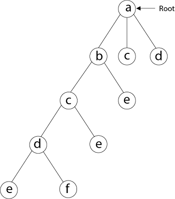
Then, adjacent to 'e,' we select vertex 'f.' D and e are the vertex next to 'f,' but they've already been there. As a result, we reach a dead end and go back a step to delete the vertex 'f' from the partial solution.

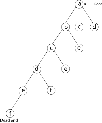
The vertices adjacent to 'e' is b, c, d, and f, from which vertex 'f' has already been verified, and b, c, and d have previously been visited, according to backtracking. As a result, we go back one step. The vertex adjacent to d is now e, f, from which e has already been checked, and the vertex adjacent to 'f' is now d and e. We get a dead state if we revisit the 'e' vertex. As a result, we go back one step.

Sum of subset

The goal of the Subset-Sum Problem is to identify a subset's' of a given set S = (S1 S2 S3...Sn), where the elements of the set S are n positive integers, such that s'S and the sum of the elements of subset's' equals some positive integer 'X.'

The backtracking method can be used to solve the Subset-Sum Problem. A binary tree is included in this implicit tree. The root of the tree is chosen to show that no decision has yet been made on any input. The items of the supplied set are assumed to be ordered in ascending order:

S1 ≤ S2 ≤ S3... ≤ Sn

The root node's left child indicated that we needed to include 'S1' from the set 'S,' and the root node's right child suggested that we needed to execute 'S1'. The total of the partial solution elements is stored in each node. If the sum equals 'X' at any point during the search, the search is complete.

The tree's dead end appears only when one of two inequalities exists:

s'+ Si + 1 > X

Example

Given a set of S = (3, 4, 5, 6) and X =9, create a new set of S = (3, 4, 5, 6) and X =9. Using the Backtracking method, find the subgroup sum.

Sol: Initially S = (3, 4, 5, 6) and X =9. 

S'= (∅) 

Figure shows the implicit binary tree for the subset sum problem:

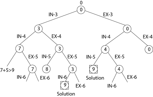
The sum of partial solution elements at a given level is the number inside a node.

Thus, if the sum of our partial solution elements equals the positive integer 'X,' the search will end at that point, or it will continue if all feasible solutions must be found.

Key takeaway

1. The root of our implicit tree is this vertex 'a.' The first intermediate vertex of the Hamiltonian Cycle to be constructed is the first element of our partial solution. By alphabetical order, the next nearby vertex is chosen.
2. The goal of the Subset-Sum Problem is to identify a subset's' of a given set S = (S1 S2 S3...Sn), where the elements of the set S are n positive integers, such that s'S and the sum of the elements of subset's' equals some positive integer 'X.'

References:

1. Thomas H. Coreman, Charles E. Leiserson and Ronald L. Rivest, “Introduction to Algorithms”, Printice Hall of India.

2. E. Horowitz & S Sahni, "Fundamentals of Computer Algorithms",

3. Aho, Hopcraft, Ullman, “The Design and Analysis of Computer Algorithms” Pearson Education, 2008.

4. LEE "Design & Analysis of Algorithms (POD)", McGraw Hill

5. Richard E.Neapolitan "Foundations of Algorithms" Jones & Bartlett Learning