Q1) What do you mean by algebraic computation?

A1) Computation in Algebra Computer algebra, also known as representational computing or algebraic computation, is a branch of computational mathematics that deals with the research and development of algorithms and software for calculating mathematical expressions and other mathematical objects.

Despite the fact that computer algebra is a subfield of scientific computing, they are commonly regarded as separate fields because scientific computing is based on numerical computation with inexact floating point numbers, whereas representational computation emphasizes exact computation with terminology that contains variables that have no given value and are manipulate as symbols, hence the name.

Q2) Explain fast and Fourier transform?

A2) The discrete Fourier transform (DFT) is a tool for converting specified types of function sequences into other sorts of representations. A fast Fourier transform (FFT) is a method that generates the discrete Fourier transform (DFT) of some sequence. Another way to put it is that the discrete Fourier transform converts the structure of a waveform's cycle into sine components.

A rapid Fourier transform can be applied to a variety of signal processing applications. It could be handy for reading sound waves or any image-processing technologies. A quick Fourier transform can be used to solve a variety of equations or to visualize various forms of frequency activity.

Fast Fourier transform and the DFT are generally the domain of engineers and mathematicians attempting to improve or develop components of various technologies, as they are an incredibly mathematical part of both computing and electrical engineering. Fast Fourier transforms, for example, could be useful in sound engineering, seismology, or voltage measurements.

The fast Fourier transform (FFT) is an algorithm that can do the discrete Fourier transform of a 2N-dimensional array in (n ln(n)) time. This algorithm is typically implemented in place, and this implementation follows suit. There are two implementations available:

●      The first implementation, FFT.basic.h, emphasizes the algorithm; as a result, it allocates additional memory when dividing the vector into even and odd entries to simplify the presentation, and it uses explicit recursion.

●      FFT.array.h, the second implementation, shows how the FFT method can be done with only O(1) additional memory and no recursive function calls.

Q3) Write short notes on string matching?

A3) The "String Searching Algorithm" is another name for the "String Matching Algorithm." "This is the approach to discover a spot where one or more strings are found within the larger string," says this important class of string algorithm.

Given a text array of n characters, T [1.....n], and a pattern array of m characters, P [1......m]. The tasks are to discover an integer s, which is referred to as valid shift, where 0 s n-m and T [s+1......s+m] = P [1......m]. To put it another way, find even if P in T, that is, if P is a substring of T.

The characters P and T are selected from a finite alphabet, such as 0 and 1 or A, B.....Z, a, b..... z. The substrings are written as T [i......j] for some 0i jn-1, the string generated by the characters in T from index I to index j, inclusive, given a string T [1......n]. This procedure determines whether or not a string is a substring of itself (assuming I = 0 and j = m).

For some 0i jn-1, the correct substring of string T [1......n] is T [1......j]. That is, either i>0 or j m-1 must be present.

We can claim that given any string T [1......n], the substrings are using these descriptions.

T [i.....j] = T [i] T [i +1] T [i+2]......T [j] for some 0≤i ≤ j≤n-1.

And correct substrings are essential.

T [i.....j] = T [i] T [i +1] T [i+2]......T [j] for some 0≤i ≤ j≤n-1. 

Q4) What kind of Algorithms used for String Matching?

A4) String matching algorithms have had a significant impact on computer science and are used to solve a variety of real-world challenges. It aids in the completion of time-saving tasks in a variety of fields. These techniques can in handy when looking for a string within another string. Database schema and network systems both employ string matching.

Let's have a look at a couple string matching algorithms before moving on to their real-world applications. Algorithms for string matching can be roughly divided into two groups.

Exact String Matching Algorithms

The goal of exact string matching algorithms is to discover one, few, or all occurrences of a specific string (pattern) in a big string (text or sequences) that are all perfect matches. All pattern alphabets must be matched to the relevant subsequence. These are further separated into four groups:

●      Naive Algorithm - It checks for a match by sliding the pattern over the text one by one. If a match is identified, slide the slider by 1 to check for more matches.

●      KMP (Knuth Morris Pratt) Algorithm - When a mismatch is found, the assumption is that we already know some of the characters in the next window's text. As a result, we use this knowledge to avoid matching characters that we already know will match.

●      Boyer Moore Algorithm - This method starts matching from the final character of the pattern and uses the best hourstics of the Naive and KMP algorithms.

●      Using the Trie data structure - It's a data structure for retrieving information quickly. The keys are stored in the form of a balanced BST.

2.     Deterministic Finite Automaton (DFA) method

●      Automaton Matcher Algorithm - It begins with the automata's first state and the first character of the text. It considers the next character of text at each step, searching for the next state in the created finite automata and moving to a new state.

3.     Algorithms based on Bit (parallelism method)

●      Aho-Corasick Algorithm - It detects all words in O(n + m + z) time, where n is the text length, m is the total number of characters in all words, and z is the total number of times a word appears in the text. The original Unix command fgrep is based on this method.

4.     Hashing-string matching algorithms:

●      Rabin Karp Algorithm - It compares the hash value of the pattern to the hash value of the current text substring, and only then does it begin matching individual characters.

Approximate String Matching Algorithms

Approximate String Matching Algorithms (sometimes called Fuzzy String Searching) look for substrings in a string. The approximate string matching approach is described in more detail as follows: Assume we have two strings, text T[1...n] and pattern P[1...m]. The goal is to discover all occurrences of patterns in the text with an edit distance of at least k from the pattern.

Q5) Describe NP completeness?

A5) NP complete class is used to solve the problems of no polynomial time algorithm.

●      If a polynomial time algorithm exists for any of these problems, all problems in NP would be polynomial time solvable. These problems are called NP-complete.

●      The phenomenon of NP-completeness is important for both theoretical and practical reasons.

●      Following are the no polynomial run time algorithm:

Application of NP complete class

●      A clique is a complete sub graph which is made by given undirected graph.

●      All the vertices are connected to each other i.e.one vertex of undirected graph is connected to all other vertices in graph.

●      There is the computational problem in clique where we can find the maximum clique of graph this known as max clique.

●      Max clique is used in many real world problems and in many application.

●      Assume a social networking where peoples are the vertices and they all are connected to each other via mutual acquaintance that becomes edges in graph.

●      In the above example clique represents a subset of people who know each other.

●      We can find max clique by taking one system which inspect all subsets.

●      But the brute force search is too time consuming for a network which has more than a few dozen vertices present in the graph.

Example:

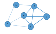
●      Let's take an example where 1, 2, 3, 4, 5, 6 are the vertices that are connected to each other in an undirected graph.

●      Here subgraph contains 2,3,4,6 vertices which form a complete graph.

●      Therefore subgraph is a clique.

●      As this is a complete subgraph of a given graph. So it’s a 4-clique.

Analysis of Clique Algorithm

●      Non deterministic algorithm uses max clique algorithm to solve problem.

●      In this algorithm we first find all the vertices in the given graph.

●      Then we check the graph is complete or not i.e. all vertices should form a complete graph.

●      The no polynomial time deterministic algorithm is used to solve this problem which is known as NP complete.

2.     Vertex Cover

●      A vertex-cover of an undirected graph G = (V, E) is a subset of vertices V' ⊆ V such that if edge (u, v) is an edge of G, then either u in V or v in V' or both.

●      In given undirected graph we need to find maximum size of vertex cover.

●      It is the optimization version of NP complete problem.

●      It is easy to find vertex cover.

Example:

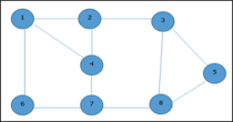
Given graph with set of edges are 

{(1,6),(1,2),(1,4),(2,3),(2,4),(6,7),(4,7),(7,8),(3,8),(3,5),(8,5)}

Now, start by selecting an edge (1, 6).

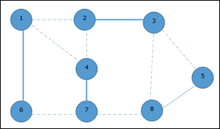
Eliminate all the edges, which are either incident to vertex 1 or 6 and we add edge (1, 6) to cover.

In the next step, we have chosen another edge (2, 3) at random

Now we select another edge (4, 7).

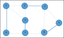
We select another edge (8, 5).

Hence, the vertex cover of this graph is {1, 2, 4, 5}.

Analysis of Vertex Cover Algorithm

●      In this algorithm, by using an adjacency list to represent E it is easy to see the running time of this algorithm is O (V+E).

Steps for proving a problems as NP-complete

First, try to prove it to be NP-hard, by :-

Significance: if anyone finds a poly algorithm for your “target” problem, then by using your poly-trans algorithm one would be able to solve that “source” NP-hard problem in poly-time, or in other words P would be = NP.

Second, try to prove that the given problem is in NP-class: by developing a polynomial algorithm for checking any "certificate" of any problem-instance.

The class P is the set of decision problems that can be solved in polynomial time.

P = {L | L ⊆ {0, 1}* and there exists an algorithm A that decides L in polynomial time}.

Q6) Write about Approximation algorithms?

A6) An Approximate Algorithm is a way of approaching the optimization problem of NP-COMPLETENESS. This approach does not guarantee the right solution. The purpose of an approximation algorithm is to get as close as possible in a reasonable amount of time to the optimum value, which is at the most polynomial moment. These algorithms are called approximation algorithms or heuristic algorithms.

An algorithm A is said to be an algorithm, given an optimization problem P.

Approximation algorithm for P if it returns an approximation algorithm for any given instance I, approximate solution, that is a feasible solution.

Types of Approximation

P An optimization problem

A An approximation algorithm

I An instance of P

A∗ (I) Optimal value for the instance I

A(I) Value for the instance I generated by A

2. Relative Approximation

Example:

1. Vertex Cover

2. Traveling Salesman Problem

3. Bin Packing

Q7) What is Randomized algorithms?

A7) Randomized Algorithms use random numbers in order to decide what should be the next step to be performed. An example of the random algorithm can be like suppose there is a group of students in class and a professor is randomly making a student stand to answer the question.

Randomized algorithms sometimes have deterministic time complexity. Algorithms like Monte Carlo algorithm use a randomized approach and its worst case complexity can be easily identified, whereas randomized algorithms like Las Vegas are dependent on the value of random variables and hence in these algorithms worst case identification becomes tougher.

In order to compute expected time taken in the worst case a time taken by every possible value needs to be evaluated. Average of all evaluated times is the expected worst case time complexity

Randomized algorithm is mainly used either to reduce the time complexity or the space complexity in the given algorithm

Randomized algorithms are classified into two categories

Example of Las Vegas

Finding Random point in the circle

It is easy and convenient to find a random point in the circle using these approach, here the idea is to first generate a point(x, y) with -1< x <1 and -1<y <1. So  if the random selected point appear in this unit circle we keep it else we will throw it and repeat until the point in the unit circle is found

Algorithm for finding Random point in the circle

Funpoint()(x,y float64)

{

For

{

x=2* rand.Float64()-1

y=2* rand.Float64()-1

If x*x+y*y < 1

{

Return

}

}

}

For example implementation of Karger’s algorithm produces a minimum cut with probability greater than or equal to (1/n2) where n is the number of vertices in Karger’s algorithm and it has the worst case time complexity as O(E).

Monte Carlo simulations are a broad class of algorithms that use repeated random sampling to obtain numerical results; these are generally used to simulate the behavior of other systems.

If a point(x, y) with -1< x <1 and -1<y <1 are placed randomly then the ratio of points that fall within the unit circle will be close to .

Algorithm to find a random point in the given circle using Monte Carlo approach

Const a = 99999

Count:= 0

For i:= 0; i <a; i++ {

x:= 2*rand.Float64() - 1

y:= 2*rand.Float64() - 1

If x*x+y*y < 1 {

Count++

}

}