Unit 1
Signals And Systems
The Advances in technology are improving capabilities of analyzing many information sources such as audio (speech, acoustics, music), image (video, multimedia, medical scans), medical signals (heart rate, blood pressure, brain activity) and remote sensing data (geophysical, radar, sonar).
Examples of systems that manipulate signals are speech recognition, video streaming, cellular networks and medical scans such as MRI.
The disciplines of signal and image processing are concerned with the analysis and synthesis of signals and their interaction with systems.
In communications, the objective is to transfer information (signals) from one or many sources to one or many destinations, which requires the design of transmission schemes (e.g., modulation and coding), receivers, and filters.
Key Takeaways:
- Signals advances in various domains.
- Applications of signal and systems
A signal is said to be energy signal when it has finite energy
Energy E =  2(t) dt
Power:
A signal is said to be power signal when it has finite power.
Power P = lim T-> ∞ 1/2T  2 (t) dt
Energy of CT signal Ex =  x(t)| 2 dt
Energy of discrete time signal Ex =  2
2
Power of CT signal Px = lim T-> ∞ 1/2T  x(t) | 2 dt
Power of DT signal Px = lim N-> ∞ 1/2N+1  2
2
Find the energy of the signal for the following diagram
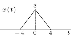
x(t) = { 3(1-t/4) if 0 
 4
4
3(1+t/4) if -4 t
t 
0 otherwise
Therefore
Ex =  x(t) | 2
(Ex =  x 2 (t) dt
= 9  2 dt +
  2 dt
2 dt
= 9. (1+t/4) 3 / ¾ | 0 -4 + 9. (1-t/4) 3 /- ¾ | 4 0
= 9 x4/3 + 9x4/3 = 24
Hence Energy Signal
Problem:
Let x(t) = A cos (wot + 
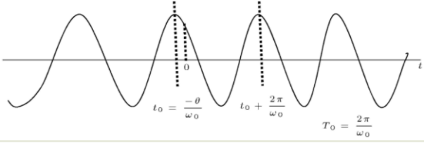
Px = 1/To  2 cos 2 (wot +
  ) dt
) dt
= 1/To  2 cos 2 (wot +
  ) dt
) dt
= A2 /To  cos (2 wot +
  )/2 dt
= A2 /To [ t/2 + sin(2wot +2 / 4wo ] –
  / wo -
  +2π/wo
=A2/T0[1/2(-0+2π/w0- -0/w0)]
=1/2*A2/T0*2π/w0
=A2/2
Continuous systems input and output continuous signals, such as analog electronics where the signal varies continuously with respect to time.
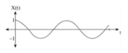
Figure 1. Continuous time signal
Discrete systems input and output discrete signals, such as computer programs that manipulate the values stored in arrays.
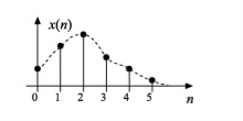
Figure 2. Discrete time signals
A continuous-time signal has values for all points in time in some (possibly infinite) interval. A discrete time signal has values for only discrete points in time.

Figure 3. Representation of continuous and discrete amplitude signals
Linearity:
Consider any two inputs on the system as follows:
X1(t) ->S-> Y1(s)
X2(t) -> S-> Y2(s)
The system is said to be linear for any two constants α and β and the signal
X(t) = α X1(t) + β X2(t)
The system acts on it as follows
X(t) -> S-> Y(s) where Y(s) = α Y1(s) + β Y2(s)
Linearity. Basically, the principle of linearity is equivalent to the principle of superposition, i.e. a system can be said to be linear if, for any two input signals, their linear combination yields as output the same linear combination of the corresponding output signals.
For example
A capacitor, an inductor, a resistor or any combination of these are all linear systems, if we consider the voltage applied across them as an input signal, and the current through them as an output signal. This is because these simple passive circuit components follow the principle of superposition within their ranges of operation.
Assume y[n] and y(t) are respectively outputs to input signals x[n] and x(t)
System with description y(t) = t. x(t) is linear.
Consider two input signals x1(t) and x2(t) with the corresponding outputs y1(t) and y2(t) where a and b are arbitrary constants. The corresponding output of ax1(t) + b x2(t) is t(ax1(t) + bx2(t))
= t ax1(t) + t b x2(t) which is the same linear combination of y1(t) and y2(t).
Suppose y(t) = |x(t)| 2
Because the system is neither additive nor homogeneous.
Additivity
Consider a system where input x1[n] produces an output y1[n]. Similarly x2[n] produces y2[n].
The system is additive when
x1[n] + x2[n] = y1[n] + y2[n]
In other words, signals added at the input will produce signals added at the output.
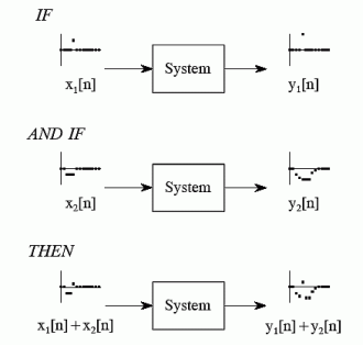
Figure 4. Addivity
Homogeneity
Homogeneity means change in input signals amplitude results in a corresponding change in the output signal’s amplitude.
That is a change in x[n] will result in a change in y [n]
Also a change in k x[n] will result in a change in k y[n]
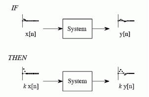
Figure 5. Homogenity
Key Takeaways:
- The properties of system.
- Importance linearity, homogeneity, and additivity
Shift Invariance
Shift invariance means that a shift in the input signal will result in an identical shift in the output signal
If x[n] -> y[n]
Then x[n+s] -> y[n +s] for any constant s
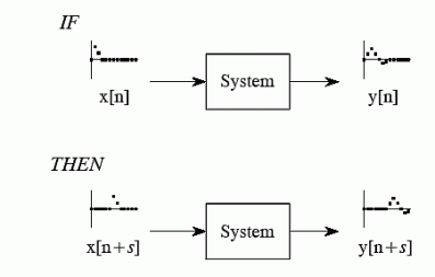
Figure 6. Shift invariance
Say, for a system, the input signal x(t) gives rise to an output signal y(t). If the input signal x(t - t0) gives rise to output y(t - t0), for every t0, and every possible input signal, we say the system is shift invariant. i.e. for every permissible x(t) and every t0
x(t) -> y(t) -> x(t-to) -> y(t-to)
In other words, for a shift invariant system, shifting the input signal shifts the output signal by the same offset.
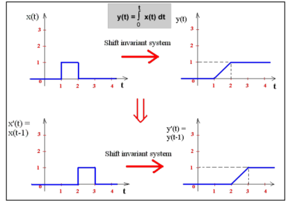
Figure.7 Shift invariant system
Key Takeaways:
- Shift invariance its definition
- Application of shift invariance
Causal signals are signals that are zero for all negative time. If any value of the output signal depends on a future value of the input signal then the signal is non-causal.
Definition:
Let x1(t) and x2(t) be two input signals to a system and y 1(t) and y2(t) be their respective outputs. The system is said to be causal if and only if:
x1(t) = x2(t) for t
y1(t) = y2( t) for t  to for every to and for every x1(t) and x2(t)
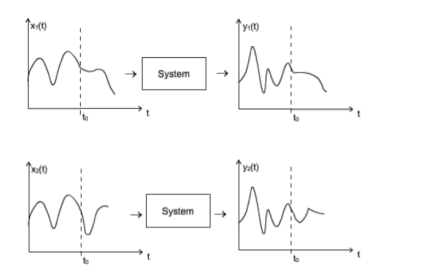
Figure 8. Casual system
Key Takeaways:
- Definition of casuality
- Derivation for casual system.
Example
Y(t) = ½[x(t) – x(-t)]
For negative values of t the output depends on future values of input
Check whether the following systems are casual or not.
y(n) = x(n) + 1/x(n-1)
For n=0
y(0) = x(0) + 1/x(0 -1)
For n=1
y(1) = x(1) + 1/ x(0)
For n=2
y(2) = y(2) + 1/x(1)
For n=-1
y(-1) = x(-1) + 1/x(-2)
For all values of n the output depends on the present and past values of input. Hence the system is casual.
- BIBO stability
Bounded input bounded output stability.
The system is BIBO stable if

A system is BIBO stable if for any bounded input signal the output signal is bounded.
Given a bounded input i.e Mx  0 |x(t)|
  Mx
Mx  t
t
My  0 |y(t)|
  My
My  t
t
It is not necessary that for input and output signal to have the same independent variable. It is valid for continuous time, discrete time and hybrid systems.
Suppose
y(t) = {x(t)} 2
If x(t) is bounded then Mx 0
0  t |x(t)|
  Mx
Mx
|y(t)|  Mx 2
Mx 2
Which further implies that the output is bounded  t
t
The system is BIBO stable
Suppose y(t) = t x(t)
Take x(t) = u(t)
Then the input is bounded by 1 and the output is bounded hence BIBO unstable.
Key Takeaways:
- Stability of the system
- Condition for stability.
In linear systems theory, the term realizability refers to the ability to characterize a known output in terms of a linear system with some input.
The regressive linear system
x ∆ = A(t)x(t) + B(t)u(t), x(t0) = 0, y(t) = C(t)x(t), of dimension n is a realization of the weighting pattern
G(t, σ(s)) if G(t, σ(s)) = C(t)ΦA(t, σ(s))B(s), for all t, s.
If a realization of this system exists, then the weighting pattern is realizable. The system is a minimal realization if no realization of G(t, σ(s)) with dimension less than n exists.
Key Take Aways:
- How to make the system realizable
- The condition for it.
References:
1. A.V. Oppenheim, A.S. Willsky and I.T. Young, "Signals and Systems," Pearson, 2015.
2. R.F. Ziemer, W.H. Tranter and D.R. Fannin, "Signals and Systems - Continuous and Discrete," 4th edition, Prentice Hall, 1998.
3. B.P. Lathi, "Signal Processing and Linear Systems," Oxford University Press, 1998.
4. Douglas K. Lindner, "Introduction to Signals and Systems," McGraw Hill International Edition: 1999.
5. Simon Haykin, Barry van Veen, "Signals and Systems," John Wiley and Sons (Asia) Private Limited, 1998.
6. V. Krishnaveni, A. Rajeswari, “"Signals and Systems," Wiley India Private Limited, 2012.
7. Robert A. Gabel, Richard A. Roberts, "Signals and Linear Systems," John Wiley and Sons, 1995.
8. M. J. Roberts, "Signals and Systems - Analysis using Transform methods and MATLAB," TMH, 2003.
9. J. Nagrath, S. N. Sharan, R. Ranjan, S. Kumar, "Signals and Systems," TMH New Delhi, 2001.
10. A. Anand Kumar, “Signals and Systems,” PHI 3rd edition, 2018.
11. D. Ganesh Rao, K.N. Hari Bhat, K. Anitha Sheela, “Signal, Systems, and Stochastic Processes,” Cengage publication, 2018