Unit-1

Random Variables

1.1 Concept of Probability

Let A and B be two events of a sample space Sand let . Then conditional probability of the event A, given B, denoted byis defined by –

Theorem: If the events A and B defined on a sample space S of a random experiment are independent, then

Example1: A factory has two machines A and B making 60% and 40% respectively of the total production. Machine A produces 3% defective items, and B produces 5% defective items. Find the probability that a given defective part came from A.

SOLUTION: We consider the following events:

A: Selected item comes from A.

B: Selected item comes from B.

D: Selected item is defective.

We are looking for . We know:

Now,

So we need

Since, D is the union of the mutually exclusive events and (the entire sample space is the union of the mutually exclusive events A and B)

Key Takeaways:

If the events A and B defined on a sample space S of a random experiment are independent, then

1.2 Random variable

A random variable (RV) X is a function from the sample space Ω to the real numbers X:Ω→R

Assuming E⊂RE⊂R we denote the event {ω∈Ω:X(ω)∈E}⊂Ωby {X∈E} or just X∈E.

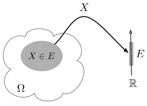
Fig.1: Random variable

1.3 Statistical averages

The mean (or average), mu, of the sample is the first moment:

 You will also see this notation sometimes

In R, the mean() function returns the average of a vector.

1.4 Random Process

A useful extension of the idea of random variables is the random process. While the random variable X is defined as a univariate function X(s) where s is the outcome of a random experiment, the random process is a bivariate function X(s, t) where s is the outcome of a random experiment and t is an index variable such as time.

Examples of random processes are the voltages in a circuit over time, light intensity over location. The random process, for two outcomes s1 and s2 can be plotted as

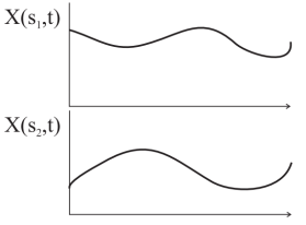
Fig.2: Random Process

Two Ways to View a Random Process

 • A random process can be viewed as a function X(t, ω) of two variables, time t ∈ T and the outcome of the underlying random experiment ω∈Ω

◦ For fixed t, X(t, ω) is a random variable over Ω

◦ For fixed ω, X(t, ω) is a deterministic function of t, called a sample function

Fig.3: Random Process

A random process is said to be discrete time if T is a countably infinite set, e.g., ◦ N = {0, 1, 2, . . .} ◦ Z = {. . . , −2, −1, 0, +1, +2, . . .}

• In this case the process is denoted by Xn, for n ∈ N, a countably infinite set, and is simply an infinite sequence of random variables

 • A sample function for a discrete time process is called a sample sequence or sample path

• A discrete-time process can comprise discrete, continuous, or mixed r.v.s

Example

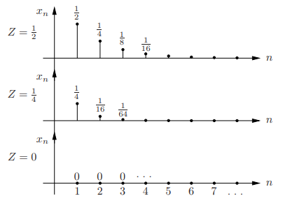
 • Let Z ∼ U[0, 1], and define the discrete time process Xn = Z n for n ≥ 1

• Sample paths:

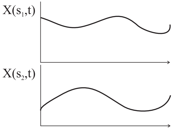
Fig.4: Sample paths

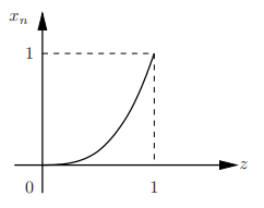
First-order pdf of the process: For each n, Xn = Z n is a r.v.; the sequence of pdfs of Xn is called the first-order pdf of the process

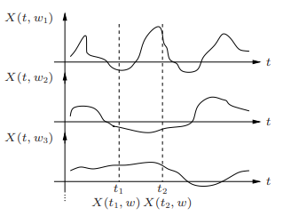
Fig.5: First-order pdf of the process

Since Xn is a differentiable function of the continuous r.v. Z, we can find its pdf as f

fXn (x) = 1/( nx(n−1)/n) = 1/n x(1/n)−1) , 0 ≤ x ≤ 1

Key Takeaways:

1. A random process can be viewed as a function X(t, ω) of two variables, time t ∈ T and the outcome of the underlying random experiment ω∈Ω

2. A sample function for a discrete time process is called a sample sequence or sample path.

1.5 Power Spectral Density & Autocorrelation Function of Random Processes

Random processes are classified according to the type of the index variable and classification of the random variables obtained from samples of the random process. The major classification is given below:

A Power Spectral Density (PSD) is the measure of signal's power content versus frequency. A PSD is typically used to characterize broadband random signals. The amplitude of the PSD is normalized by the spectral resolution employed to digitize the signal.

For vibration data, a PSD has amplitude units of g2/Hz. While this unit may not seem intuitive at first, it helps ensure that random data can be overlaid and compared independently of the spectral resolution used to measure the data. 

The average power {\displaystyle P}P of a signal {\displaystyle x(t)}x(t) over all time is therefore given by the following time average:

1.6 Gaussian Random Process

It is a stochastic process (a collection of random variables indexed by time or space), such that every finite collection of those random variables has a multivariate normal distribution, i.e. every finite linear combination of them is normally distributed. The distribution of a Gaussian process is the joint distribution of all those (infinitely many) random variables, and as such, it is a distribution over functions with a continuous domain, e.g. time or space.

A random process {X(t),t∈J}{X(t),t∈J} is said to be a Gaussian (normal) random process if, for all

t1,t2,…,tn∈J,t1,t2,…,tn∈J,

the random variables X(t1)X(t1), X(t2)X(t2),..., X(tn)X(tn) are jointly normal.

Numerical:

Let X(t) be a zero-mean WSS Gaussian process with RX(τ)=e−τ2, for all τ∈R.

Solution:

Var(X(1))=E[X(1)2]=RX(0)=1.

Thus,

P(X(1)<1)=Φ(1−01)=Φ(1)≈0.84

2.     Let Y=X(1)+X(2)Y=X(1)+X(2). Then, YY is a normal random variable. We have

EY=E[X(1)]+E[X(2)]=0;

Var(Y)=Var(X(1))+Var(X(2))+2Cov(X(1),X(2)).

Note that

Var(X(1))=E[X(1)2]−E[X(1)]2=RX(0)−μ2X=1−0=1=Var(X(2));

Cov(X(1),X(2))=E[X(1)X(2)]−E[X(1)]E[X(2)]=RX(−1)−μ2X=e−1−0=1e

Therefore,

Var(Y)=2+2e.

We conclude Y∼N(0,2+2e). Thus,

P(Y<1)= Φ ()

=Φ(0.6046)≈0.73

References:

1. B.P. Lathi, “Modern Digital and Analog communication Systems”, 4th Edition, Oxford

University Press.

2. John G. Proakis, “Digital Communications”, 5th Edition, TMH.

3. H. Taub, D L Schilling, Gautam Saha, “Principles of Communication”, 4th Edition,

TMH.

4. Singh & Sapray, Communication Systems, 3th Edition, TMH.