Unit 5
Statistical techniques-3
Population-
The population is the collection or group of observations under study.
The total number of observations in a population is known as population size, and it is denoted by N.
Types of the population-
Sample –
To extract the information from all the elements or units or items of a large population may be, in general, time-consuming, expensive, and difficult., and also if the elements or units of the population are destroyed under investigation then gathering the information from all the units is not make a sense. For example, to test the blood, doctors take a very small amount of blood. Or to test the quality of a certain sweet we take a small piece of sweet. In such situations, a small part of the population is selected from the population which is called a sample
Complete survey-
When each, and every element or unit of the population is investigated or studied for the characteristics under study then we call it a complete survey or census.
Sample Survey
When only a part of a small number of elements or units (i.e. sample) of the population are investigated or studied for the characteristics under study then we call it sample survey or sample enumeration Simple Random Sampling or Random Sampling
The simplest and most common method of sampling is simple random sampling. In simple random sampling, the sample is drawn in such a way that each element or unit of the population has an equal, and independent chance of being included in the sample. If a sample is drawn by this method then it is known as a simple random sample or random sample
Simple Random Sampling without Replacement (SRSWOR)
In simple random sampling, if the elements or units are selected or drawn one by one in such a way that an element or unit drawn at a time is not replaced to the population before the subsequent draws are called SRSWOR.
Suppose we draw a sample from a population, the size of the sample is n, and the size of the population is N, then the total number of possible sample is 
Simple Random Sampling with Replacement (SRSWR)
In simple random sampling, if the elements or units are selected or drawn one by one in such a way that a unit drawn at a time is replaced to the population before the subsequent draw is called SRSWR.
Suppose we draw a sample from a population, the size of the sample is n, and the size of the population is N, then the total number of possible sample is  .
.
Parameter-
A parameter is a function of population values which is used to represent the certain characteristic of the population. For example, population mean, population variance, population coefficient of variation, population correlation coefficient, etc. are all parameters. Population parameter mean usually denoted by μ, and population variance denoted by 
The sample mean, and sample variance-
Let  be a random sample of size n taken from a population whose pmf or pdf function f(x,
Then the sample mean is defined by-

And sample variance-

Statistic-
Any quantity which does not contain any unknown parameter, and calculated from sample values is known as a statistic.
Suppose  is a random sample of size n taken from a population with mean μ, and variance
  then the sample mean-

Is a statistic.
Estimator, and estimate-
if a statistic is used to estimate an unknown population parameter then it is known as an estimator, and the value of the estimator based on the observed value of the sample is known as an estimate of the parameter.
Hypothesis-
A hypothesis is a statement or a claim or an assumption about the value of a population parameter (e.g., mean, median, variance, proportion, etc.).
Similarly, in the case of two or more populations, a hypothesis is a comparative statement or a claim, or an assumption about the values of population parameters. (e.g., means of two populations are equal, the variance of one population is greater than other, etc.).
For example-
If a customer of a car wants to test whether the claim of the car of a certain brand gives the average of 30km/hr is true or false.
Simple, and composite hypotheses-
If a hypothesis specifies only one value or exact value of the population parameter then it is known as a simple hypothesis., and if a hypothesis specifies not just one value but a range of values that the population parameter may assume is called a composite hypothesis.
The null, and alternative hypothesis
The hypothesis is to be tested as called the null hypothesis.
The hypothesis which complements the null hypothesis is called the alternative hypothesis.
In the example of a car, the claim is  , and its complement is
  .
.
The null and alternative hypothesis can be formulated as-

And

Critical region-
Let  be a random sample drawn from a population having unknown population parameter
  .
.
The collection of all possible values of  is called sample space, and a particular value represents a point in that space.
To test a hypothesis, the entire sample space is partitioned into two disjoint sub-spaces, say,  , and S –
  . If the calculated value of the test statistic lies in, then we reject the null hypothesis, and if it lies in
  then we do not reject the null hypothesis. The region is called a “rejection region or critical region”, and the region
  is called a “non-rejection region”.
Therefore, we can say that
“A region in the sample space in which if the calculated value of the test statistic lies, we reject the null hypothesis then it is called a critical region or rejection region.”
The region of rejection is called the critical region.
The critical region lies in one or two tails on the probability curve of the sampling distribution of the test statistic it depends on the alternative hypothesis.
Therefore, there are three cases-
CASE-1: if the alternative hypothesis is right-sided such as  then the entire critical region of size
  lies on the right tail of the probability curve.
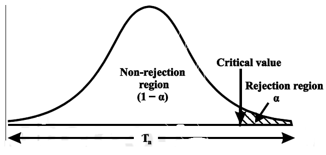
CASE-2: if the alternative hypothesis is left-sided such as  then the entire critical region of size
  lies on the left tail of the probability curve.
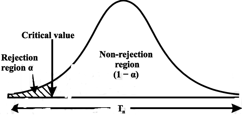
CASE-3: if the alternative hypothesis is two-sided such as  then the entire critical region of size
  lies on both tail of the probability curve
Type-1, and Type-2 error-
Type-1 error-
The decision relating to the rejection of null hypo. When it is true is called a type-1 error.
The probability of type-1 error is called the size of the test, it is denoted by  , and defined as-

Note-
 is the probability of a correct decision.
Type-2 error-
The decision relating to the non-rejection of null hypo. When it is false is called a type-1 error.
It is denoted by  defined as-

Decision | |
|
Reject | Type-1 error | Correct decision |
Do not reject | Correct decision | Type-2 error |
One-tailed, and two-tailed tests-
A test of testing the null hypothesis is said to be a two-tailed test if the alternative hypothesis is two-tailed whereas if the alternative hypothesis is one-tailed then a test of testing the null hypothesis is said to be a one-tailed test.
For example, if our null and alternative hypothesis are-

then the test for testing the null hypothesis is two-tailed because the
an alternative hypothesis is two-tailed.
If the null and alternative hypotheses are-

then the test for testing the null hypothesis is right-tailed because the alternative hypothesis is right-tailed.
Similarly, if the null and alternative hypotheses are-

then the test for testing the null hypothesis is left-tailed because the alternative hypothesis is left-tailed
Procedure for testing a hypothesis-
Step-1: first we set up the null hypothesis  , and alternative hypothesis
  .
.
Step-2: After setting the null, and alternative hypothesis, we establish
criteria for rejection or non-rejection of the null hypothesis, that is,
decide the level of significance ( ), at which we want to test our
hypothesis. Generally, it is taken as 5% or 1% (α = 0.05 or 0.01).
step-3: The third step is to choose an appropriate test statistic under H0 for
testing the null hypothesis as given below

Now after doing this, specify the sampling distribution of the test statistic preferably in the standard form like Z (standard normal),  , t, F or any other well-known in the literature
Step-4: Calculate the value of the test statistic described in Step III based on observed sample observations.
Step-5: Obtain the critical (or cut-off) value(s) in the sampling distribution of the test statistic, and construct rejection (critical) region of size  .
.
Generally, critical values for various levels of significance are put in the form of a table for various standard sampling distributions of test statistic such as Z-table,  -table, t-table, etc
Step-6: After that, compare the calculated value of the test statistic obtained from Step IV, with the critical value(s) obtained in Step V, and locates the position of the calculated test statistic, that is, it lies in the rejection region or non-rejection region.
Step-7: in testing the hypothesis we have to conclude, it is performed as below-
First- If the calculated value of the test statistic lies in the rejection region at  level of significance then we reject the null hypothesis. It means that the sample data provide us sufficient evidence against the null hypothesis, and there is a significant difference between the hypothesized value and the observed value of the parameter
Second- If the calculated value of the test statistic lies in the non-rejection region at  level of significance then we do not reject the null hypothesis. Its means that the sample data fails to provide us sufficient evidence against the null hypothesis, and the difference between hypothesized value, an observed value of the parameter due to fluctuation of sample
The procedure of testing of hypothesis for large samples-
A sample size of more than 30 is considered a large sample size. So that for large samples, we follow the following procedure to test the hypothesis.
Step-1: first we set up the null and alternative hypothesis.
Step-2: After setting the null, and alternative hypotheses, we have to choose the level of significance. Generally, it is taken as 5% or 1% (α = 0.05 or 0.01)., and accordingly rejection and non-rejection regions will be decided.
Step-3: The third step is to determine an appropriate test statistic, say, Z in the case of large samples. Suppose Tn is the sample statistic such as sample
mean, sample proportion, sample variance, etc. for the parameter 
then for testing the null hypothesis, the test statistic is given by

Step-4: the test statistic Z will assumed to be approximately normally distributed with mean 0, and variance 1 as

By putting the values in the above formula, we calculate test statistic Z.
Suppose z be the calculated value of Z statistic
Step-5: After that, we obtain the critical (cut-off or tabulated) value(s) in the sampling distribution of the test statistic Z corresponding to  assumed in Step II. we construct the rejection (critical) region of size α in the probability curve of the sampling distribution of test statistic Z.
Step-6: Decide on the null hypothesis based on the calculated, and critical values of test statistic obtained in Step IV, and Step V.
Since critical value depends upon the nature of the test that it is a one-tailed test or two-tailed test so following cases arise-
Case-1 one-tailed test- when  (right-tailed test)
In this case, the rejection (critical) region falls under the right tail of the probability curve of the sampling distribution of test statistic Z.
Suppose  is the critical value at
  level of significance so the entire region greater than or equal to
  is the rejection region, and less than
 is the non-rejection region
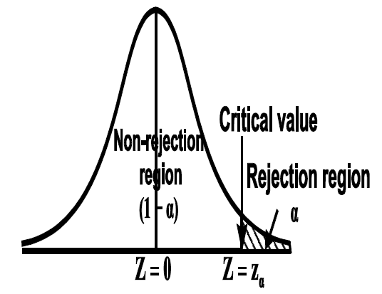
If z (calculated value ) ≥  (tabulated value), that means the calculated value of test statistic Z lies in the rejection region, then we reject the null hypothesis H0 at
  level of significance. Therefore, we conclude that sample data provides us sufficient evidence against the null hypothesis, and there is a significant difference between the hypothesized or specified value, and the observed value of the parameter.
If z < that means the calculated value of test statistic Z lies in the non-rejection region, then we do not reject the null hypothesis H0 at
  level of significance. Therefore, we conclude that the sample data fails to provide us sufficient evidence against the null hypothesis, and the difference between hypothesized value, an observed value of the parameter due to fluctuation of the sample.
So the population parameter 
Case-2: when  (left-tailed test)
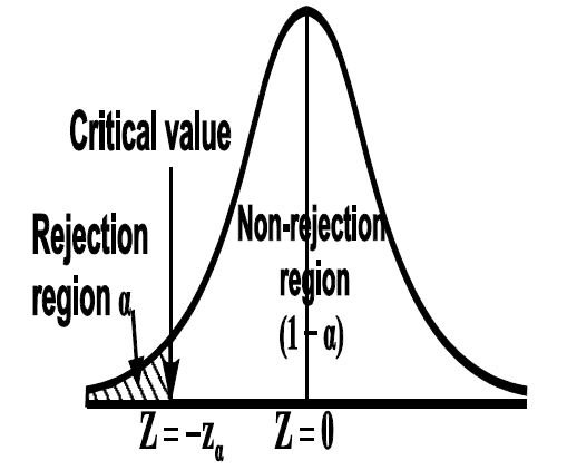
the rejection (critical) region falls under the left tail of the probability curve of the sampling distribution of test statistic Z.
Suppose - is the critical value at
  level of significance than the entire region less than or equal to -
 is the rejection region, and greater than -
 is the non-rejection region
If z ≤- , that means the calculated value of test statistic Z lies in the rejection region, then we reject the null hypothesis H0 at
  level of significance.
If z >- , that means the calculated value of test statistic Z lies in the non-rejection region, then we do not reject the null hypothesis H0 at
  level of significance.
In the case of the two-tailed test-

In this case, the rejection region falls under both tails of the probability curve of the sampling distribution of the test statistic Z. Half the area (α) i.e. α/2 will lie under the left tail, and the other half under the right tail. Suppose  , and
, and  are the two critical values at the left-tailed, and right-tailed respectively. Therefore, an entire region less than or equal to
  and greater than or equal to
  are the rejection regions, and between -
 is the non-rejection region.
If Z that means the calculated value of test statistic Z lies in the rejection region, then we reject the null hypothesis H0 at
  level of significance.
If  that means the calculated value of test statistic Z lies in the non-rejection region, then we do not reject the null hypothesis H0 at
  level of significance.
Testing of hypothesis for the population mean using Z-Test
For testing the null hypothesis, the test statistic Z is given as-
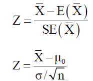
The sampling distribution of the test statistics depends upon variance 
So that there are two cases-
Case-1: when  is known -
The test statistic follows the normal distribution with mean 0, and variance unity when the sample size is large as the population under study is normal or non-normal. If the sample size is small then test statistic Z follows the normal distribution only when the population under study is normal. Thus,

Case-1: when  is unknown –
We estimate the value of  by using the value of sample variance

Then the test statistic becomes-

After that, we calculate the value of the test statistic as may be the case ( is known or unknown), and compare it with the critical value at the prefixed level of significance α.
Example: A manufacturer of ballpoint pens claims that a certain pen manufactured by him has a mean writing-life of at least 460 A-4 size pages. A purchasing agent selects a sample of 100 pens and put them on the test. The mean writing-life of the sample found 453 A-4 size pages with a standard deviation of 25 A-4 size pages. Should the purchasing agent reject the manufacturer’s claim at a 1% level of significance?
Sol.
It is given that-
The specified value of the population mean =  = 460,
Sample size = 100
Sample mean = 453
Sample standard deviation = S = 25
The null, and alternative hypothesis will be-

Also, the alternative hypothesis left-tailed so that the test is left tailed test.
Here, we want to test the hypothesis regarding population mean when population SD is unknown. So we should use a t-test for if the writing-life of the pen follows a normal distribution. But it is not the case. Since sample size is n = 100 (n > 30) large so we go for Z-test. The test statistic of Z-test is given by


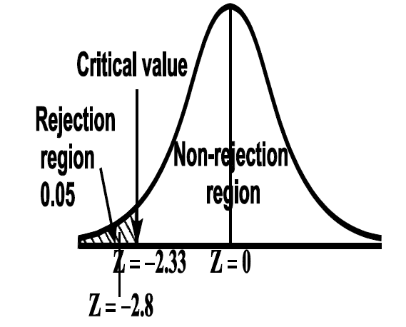
We get the critical value of left tailed Z test at 1% level of significance is 
Since the calculated value of test statistic Z (= ‒2.8,) is less than the critical value
(= −2.33), that means the calculated value of test statistic Z lies in the rejection region so we reject the null hypothesis. Since the null hypothesis is the claim so we reject the manufacturer’s claim at a 1% level of significance.
Example: A big company uses thousands of CFL lights every year. The brand that the company has been using in the past has an average life of 1200 hours. A new brand is offered to the company at a price lower than they are paying for the old brand. Consequently, a sample of 100 CFL light of new brand is tested which yields an average life of 1220 hours with a standard deviation of 90 hours. Should the company accept the new brand at a 5% level of significance?
Sol.
Here we have-

The company may accept the new CFL light when the average life of
CFL light is greater than 1200 hours. So the company wants to test that the new brand CFL light has an average life greater than 1200 hours. So our claim is  > 1200, and its complement is
  ≤ 1200. Since complement contains the equality sign so we can take the complement as the null hypothesis, and the claim as the alternative hypothesis. Thus,

Since the alternative hypothesis is right-tailed so the test is right-tailed.
Here, we want to test the hypothesis regarding population mean when population SD is unknown, so we should use a t-test if the distribution of life of bulbs known to be normal. But it is not the case. Since the sample size is large (n > 30) so we can go for a Z-test instead of a t-test.
Therefore, the test statistic is given by


The critical values for a right-tailed test at a 5% level of significance is
 1.645
1.645
Since the calculated value of test statistic Z (= 2.22) is greater than the critical value (= 1.645), that means it lies in the rejection region so we reject the null hypothesis, and support the alternative hypothesis i.e. we support our claim at a 5% level of significance
Thus, we conclude that the sample does not provide us sufficient evidence against the claim so we may assume that the company accepts the new brand of bulbs
Level of significance-
The probability of type-1 error is called the level of significance of a test. It is also called the size of the test or the size of the critical region. Denoted by  .
.
It is prefixed as a 5% or 1% level of significance.
If the calculated value of the test statistics lies in the critical region then we reject the null hypothesis.
The level of significance relates to the trueness of the conclusion. If the null hypothesis does not reject at level 5% then a person will be sure “concluding about the null hypothesis” is true with 95% assurance but even it may false with 5% chance.
Significance test of the difference between sample means
Given two independent examples  , and
, and  with means
  standard derivations
  from a normal population with the same variance, we have to test the hypothesis that the population means
  are same For this, we calculate


It can be shown that the variate t defined by (1) follows the t distribution with  degrees of freedom.
If the calculated value  the difference between the sample means is said to be significant at a 5% level of significance.
If  , the difference is said to be significant at a 1% level of significance.
If  the data is said to be consistent with the hypothesis that
  .
.
Cor. If the two samples are of the same size, and the data are paired, then t is defined by

 =difference of the ith member of the sample
d=mean of the differences = , and the member of d.f.=n-1.
Example
Eleven students were given a test in statistics. They were given a month’s further tuition, and the second test of equal difficulty was held at the end of this. Do the marks give evidence that the students have benefitted from extra coaching?
Boys | 1 | 2 | 3 | 4 | 5 | 6 | 7 | 8 | 9 | 10 | 11 |
Marks I test | 23 | 20 | 19 | 21 | 18 | 20 | 18 | 17 | 23 | 16 | 19 |
Marks II test | 24 | 19 | 22 | 18 | 20 | 22 | 20 | 20 | 23 | 20 | 17 |
Sol. We compute the mean, and the S.D. of the difference between the marks of the two tests as under:

Assuming that the students have not been benefitted by extra coaching, it implies that the mean of the difference between the marks of the two tests is zero i.e.
Then,  nearly, and df v=11-1=10
Students |
|
|
|
|
|
1 | 23 | 24 | 1 | 0 | 0 |
2 | 20 | 19 | -1 | -2 | 4 |
3 | 19 | 22 | 3 | 2 | 4 |
4 | 21 | 18 | -3 | -4 | 16 |
5 | 18 | 20 | 2 | 1 | 1 |
6 | 20 | 22 | 2 | 1 | 1 |
7 | 18 | 20 | 2 | 1 | 1 |
8 | 17 | 20 | 3 | 2 | 4 |
9 | 23 | 23 | - | -1 | 1 |
10 | 16 | 20 | 4 | 3 | 9 |
11 | 19 | 17 | -2 | -3 | 9 |
|
|
|
|
|
|
we find that  (for v=10) =2.228. As the calculated value of
  , the value of t is not significant at a 5% level of significance i.e. the test provides no evidence that the students have benefitted by extra coaching.
Example:
From a random sample of 10 pigs fed on diet A, the increase in weight in certain period were 10,6,16,17,13,12,8,14,15,9 lbs. For another random sample of 12 pigs fed on diet B, the increase in the same period were 7,13,22,15,12,14,18,8,21,23,10,17 lbs. Test whether diets A and B differ significantly as regards their effect on weight increases?
Sol. We calculate the means, and standard derivations of the samples as follows
| Diet A |
|
| Diet B |
|
|
|
|
|
|
|
10 | -2 | 4 | 7 | -8 | 64 |
6 | -6 | 36 | 13 | -2 | 4 |
16 | 4 | 16 | 22 | 7 | 49 |
17 | 5 | 25 | 15 | 0 | 0 |
13 | 1 | 1 | 12 | -3 | 9 |
12 | 0 | 0 | 14 | -1 | 1 |
8 | -4 | 16 | 18 | 3 | 9 |
14 | 2 | 4 | 8 | -7 | 49 |
15 | 3 | 9 | 21 | 6 | 36 |
9 | -3 | 9 | 23 | 8 | 64 |
|
|
| 10 | -5 | 25 |
|
|
| 17 | 2 | 4 |
|
|
|
|
|
|
120 |
|
| 180 | 0 | 314 |


Assuming that the samples do not differ in weight so far as the two diets are concerned i.e. 


For v=20, we find  =2.09
=2.09
The calculated value of 
Hence the difference between the sample's means is not significant i.e. the two diets do not differ significantly as regards their effects on the increase in weight.
Testing of hypothesis for the difference of two population means using Z-Test-
Let there be two populations, say, population-I, and population-II under study.
Also, let  denote the means, and variances of population-I, and population-II respectively where both
  are unknown but
  maybe known or unknown. We will consider all possible cases here. For testing the hypothesis about the difference between two population means, we draw a random sample of large size n1 from population-I, and a random sample of large size n2 from population-II. Let
  be the means of the samples selected from population-I, and II respectively.
These two populations may or may not be normal but according to the central limit theorem, the sampling distribution of difference of two large sample means asymptotically normally distributed with mean  , and variance

And

We know that the standard error = 

Here, we want to test the hypothesis about the difference between two population means so we can take the null hypothesis as

Or

And the alternative hypothesis is-


Or

The test statistic Z is given by-

Or
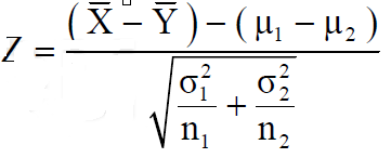
Since under the null hypothesis, we assume that  , therefore, we get-
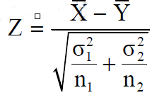
Now, the sampling distribution of the test statistic depends upon  that both are known or unknown. Therefore, four cases arise-
Case-1: When  are known, and
In this case, the test statistic follows a normal distribution with mean
0, and variance unity when the sample sizes are large as both the populations under study are normal or non-normal. But when sample sizes are small then test statistic Z follows normal distribution only when populations under study are normal, that is,
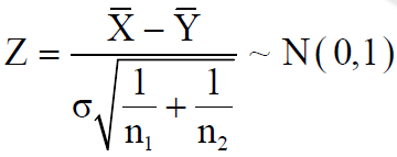
Case-2: When  are known, and
In this case, the test statistic also follows the normal distribution as described in case I, that is,
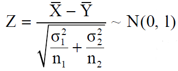
Case-3: When  are unknown, and
In this case, σ2 is estimated by the value of pooled sample variance 
where,


and test statistic follows t-distribution with (n1 + n2 − 2) degrees of freedom as the sample sizes are large or small provided populations under study follow a normal distribution.
But when the populations are under study are not normal, and sample sizes n1, and n2are large (> 30) then by central limit theorem, test statistic approximately normally distributed with mean
0, and variance unity, that is,
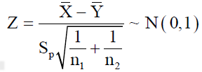
Case-4: When  are unknown, and
In this case,  are estimated by the values of the sample variances
  respectively, and the exact distribution of test statistics is difficult to derive. But when sample sizes n1, and n2 are large (> 30) than the central limit theorem, the test statistic approximately normally distributed with mean 0, and variance unity,
that is,
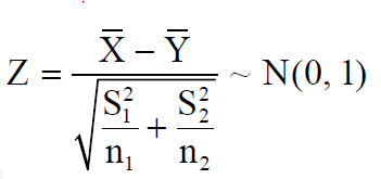
After that, we calculate the value of the test statistic and compare it with the critical value at the prefixed level of significance α.
Example: A college conducts both face-to-face, and distance mode classes for a particular course intended both to be identical. A sample of 50 students of face to face mode yields examination results mean, and SD respectively as-

and other samples of 100 distance-mode students yields mean, and SD of their examination results in the same course respectively as:

Are both educational methods statistically equal at the 5% level?
Sol. here we have-

Here we wish to test that both educational methods are statistically equal. If  denote the average marks of face to face, and distance mode students respectively then our claim is
  , and its complement is
  ≠
≠  . Since the claim contains the equality sign so we can take the claim as the null hypothesis, and complement as the alternative hypothesis. Thus,

Since the alternative hypothesis is two-tailed so the test is two-tailed.
We want to test the null hypothesis regarding two population means when standard deviations of both populations are unknown. So we should go for a t-test if the population of difference is known to be normal. But it is not the case.
Since sample sizes are large (n1, and n2 > 30) so we go for Z-test.
For testing the null hypothesis, the test statistic Z is given by


The critical (tabulated) values for a two-tailed test at a 5% level of significance are-

Since the calculated value of Z ( = 2.23) is greater than the critical values
(= ±1.96), that means it lies in the rejection region so we
reject the null hypothesis i.e. we reject the claim at a 5% level of significance
The general procedure of t-test for testing hypothesis-
Let X1, X2,…, Xn be a random sample of small size n (< 30) selected from a normal population, having parameter of interest, say,
which is unknown but its hypothetical value- then
Step-1: First of all, we set up null and alternative hypotheses
Step-2: After setting the null, and alternative hypotheses our next step is to decide criteria for rejection or non-rejection of null hypothesis i.e. decide the level of significance  at which we want to test our null hypothesis. We generally take
 = 5 % or 1%.
Step-3: The third step is to determine an appropriate test statistic, say, t for testing the null hypothesis. Suppose Tn is the sample statistic (maybe sample mean, sample correlation coefficient, etc. depending upon  ) for the parameter
  then test-statistic t is given by

Step-4: As we know, the t-test is based on t-distribution, and t-distribution is described with the help of its degrees of freedom, therefore, test statistic t follows t-distribution with specified degrees of freedom as the case may be.
By putting the values of Tn, E(Tn), and SE(Tn) in the above formula, we calculate the value of test statistic t. Let t-cal be the calculated value of test statistic t after putting these values.
Step-5: After that, we obtain the critical (cut-off or tabulated) value(s) in the sampling distribution of the test statistic t corresponding to assumed in Step II. The critical values for the t-test are corresponding to a different level of significance (α). After that, we construct the rejection (critical) region of size
  in the probability curve of the sampling distribution of test statistic t.
Step-6: Decide on the null hypothesis based on calculated, and critical value(s) of test statistic obtained in Step IV, and Step V respectively.
Critical values depend upon the nature of the test.
The following cases arise-
In the case of the one-tailed test-
Case-1:  [Right-tailed test]
In this case, the rejection (critical) region falls under the right tail of the probability curve of the sampling distribution of test statistic t.
Suppose  is the critical value at
  level of significance than the entire region greater than or equal to
  is the rejection region, and less than
  is the non-rejection region.
If  ≥
≥ that means the calculated value of test statistic t lies in the rejection (critical) region, then we reject the null hypothesis
  at
at  level of significance.
If  <
< that means the calculated value of test statistic t lies in the non-rejection region, then we do not reject the null hypothesis
  at
at  level of significance.
Case-2:  [Left-tailed test]
In this case, the rejection (critical) region falls under the left tail of the probability curve of the sampling distribution of test statistic t.
Suppose - is the critical value at
  level of significance than the entire region less than or equal to -
 is the rejection region, and greater than -
 is the non-rejection region.
If ≤ −
≤ − that means the calculated value of test statistic t lies in the rejection (critical) region, then we reject the null hypothesis
  at
at  level of significance.
If  > −
> − , that means the calculated value of test statistic t lies in the non-rejection region, then we do not reject the null hypothesis
  at
at  level of significance.
In the case of the two-tailed test-

In this case, the rejection region falls under both tails of the probability curve of the sampling distribution of the test statistic t. half the area (α) i.e. α/2 will lie under the left tail, and another half under the right tail. Suppose - , and
, and  are the two critical values at the left- tailed, and right-tailed respectively. Therefore, an entire region less than or equal to -
 and greater than or equal to
  are the rejection regions, and between -
 and
and  is the non-rejection region.
If  ≥
≥  or
or  ≤ -
≤ - , that means the calculated value of test statistic t lies in the rejection(critical) region, then we reject the null hypothesis
  at
at level of significance.
And if - <
<  <
<  , that means the calculated value of test statistic t lies in the non-rejection region, then we do not reject the null hypothesis
  at
at  level of significance.
Testing of hypothesis for the population mean using t-Test
There are the following assumptions of the t-test-

For testing the null hypothesis, the test statistic t is given by-

Example: A tyre manufacturer claims that the average life of a particular category
of his tyre is 18000 km when used under normal driving conditions. A random sample of 16 tyres was tested. The mean, and SD of life of the tyres in the sample were 20000 km, and 6000 km respectively.
Assuming that the life of the tyres is normally distributed, test the claim of the manufacturer at a 1% level of significance using the appropriate test.
Sol.
Here we have-

we want to test that manufacturer’s claim is true that the average
life ( ) of tyres is 18000 km. So claim is μ = 18000, and its complement
is μ ≠ 18000. Since the claim contains the equality sign so we can take
the claim as the null hypothesis, and complement as the alternative
hypothesis. Thus,


Here, population SD is unknown, and the population under study is given to
be normal.
So here can use t-test-
For testing the null hypothesis, the test statistic t is given by-

The critical value of test statistic t for two-tailed test corresponding (n-1) = 15 df at 1% level of significance are 
Since the calculated value of test statistic t (= 1.33) is less than the critical (tabulated) value (= 2.947), and greater than the critical value (= − 2.947), that means the calculated value of test statistic lies in the non-rejection region, so we do not reject the null hypothesis. we conclude that the sample fails to provide sufficient evidence against the claim so we may assume that manufacturer’s claim is true.
F-test-
Assumption of F-test-
The assumptions for F-test for testing the variances of two populations are:
Let  be a random sample of size
  taken from a normal population with
  variance
  be a random sample of size
  from another normal population with a mean
  , and
, and  .
.
Here, we want to test the hypothesis about the two population variances so we can take our alternative null, and hypotheses as-
For two-tailed test-

For one-tailed test-

We use test statistic F for testing the null hypothesis-


And

In the case of the one-tailed test-
Case-1:  (right-tailed test)
In this case, the rejection (critical) region falls at the right side of the probability curve of the sampling distribution of test statistic F. suppose  is the critical value of test statistic F with (
 =
=  – 1,
– 1,  =
=  – 1) df at
  level of significance so entire region greater than or equal
  to is the rejection (critical) region, and less than
  is the non-rejection region.
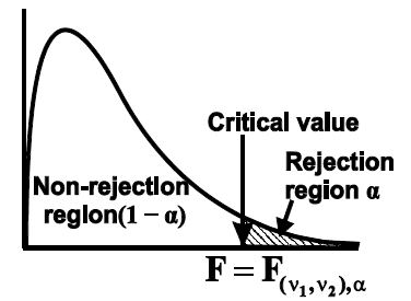
If  that means the calculated value of the test statistic lies in the rejection (critical) region, then we reject the null hypothesis H0 at
 level of significance. Therefore, we conclude that samples data provide us sufficient evidence against the null hypothesis, and there is a significant difference between population variances
If  , that means the calculated value of the test statistic lies in the non-rejection region, then we do not reject the null hypothesis H0 at
  level of significance. Therefore, we conclude that the sample data fail to provide us sufficient evidence against the null hypothesis, and the difference between population variances due to fluctuation of the sample.
Case-2:  (left-tailed test)
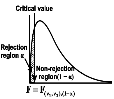
In this case, the rejection (critical) region falls at the left side of the probability curve of the sampling distribution of test statistic F. suppose  is the critical value at
 level of significance than the entire region less than or equal to
  is the rejection(critical) region, and greater than
  is the non-rejection region.
If  that means the calculated value of the test statistic lies in the rejection (critical) region, then we reject the null hypothesis H0 at
  level of significance.
If  that means the calculated value of the test statistic lies in the non-rejection region, then we do not reject the null hypothesis H0 at
  level of significance.
In the case of the two-tailed test-
When 
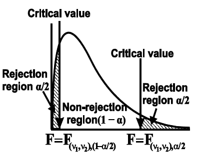
In this case, the rejection (critical) region falls at both sides of the probability curve of the sampling distribution of test statistic F, and half the area(α) i.e. α/2 of rejection (critical) region lies at the left tail and another half on the right tail.
Suppose  and
and  are the two critical values at the left-tailed, and right-tailed respectively on pre-fixed
 level of significance. Therefore, an entire region less than or equal to
  , and greater than or equal to
  are the rejection (critical) regions, and between
  , and
, and  is the non-rejection region
If  or
or  that means the calculated value of the test statistic lies in the rejection(critical) region, then we reject the null hypothesis H0 at the α level of significance.
If  that means the calculated value of test statistic F lies in the non-rejection region, then we do not reject the null hypothesis H0 at α level of significance.
Example: Two sources of raw materials are under consideration by a bulb manufacturing company. Both sources seem to have similar characteristics but the company is not sure about their respective uniformity. A sample of 12 lots from source A yields a variance of 125, and a sample of 10 lots from source B yields a variance of 112. Is it likely that the variance of source A significantly differs from the variance of source B at significance level α = 0.01?
Sol.

The null, and alternative hypothesis will be-

Since the alternative hypothesis is two-tailed so the test is two-tailed.
Here, we want to test the hypothesis about two population variances and sample sizes  = 12(< 30), and
  = 10 (< 30) are small. Also, the populations under study are normal, and both samples are independent.
so we can go for F-test for two population variances.
The test statistic is-


The critical (tabulated) value of test statistic F for the two-tailed test corresponding  = (11, 9) df at 5% level of significance are
  , and
, and

Since the calculated value of test statistic (= 1.11) is less than the critical value (= 3.91), and greater than the critical value (= 0.28), that means the calculated value of test statistic lies in the non-rejection region, so we do not reject the null hypothesis, and reject the alternative hypothesis. we conclude that samples provide us sufficient evidence against the claim so we may assume that the variances of source A and B differ.
Chi-square  test
test
When a fair coin is tossed 80 times we expect from the theoretical considerations that heads will appear 40 times, and tail 40 times. But this never happens in practice that is the results obtained in an experiment do not agree exactly with the theoretical results. The magnitude of discrepancy between observations, and theory is given by the quantity  (pronounced as chi-squares). If
  the observed, and theoretical frequencies completely agree. As the value of
  increases, the discrepancy between the observed, and theoretical frequencies increases.
Definition. If  , and
, and  be the corresponding set of expected (theoretical) frequencies, then
  is defined by the relation


Chi-square distribution
If  be n independent normal variates with mean zero, and s.d. unity, then it can be shown that
  is a random variate having
  distribution with ndf.
The equation of the  curve is

(1) Properties of  distribution


 have been tabulated for various values of P, and values of v from 1 to 30. (Table V Appendix 2)
 , the
, the curve approximates to the normal curve, and we should refer to normal distribution tables for significant values of
  .
.
IV. Since the equation of  the curve does not involve any parameters of the population, this distribution does not dependent on the form of the population.
V. Mean =  , and variance =
Goodness of fit
The values of  is used to test whether the deviations of the observed frequencies from the expected frequencies are significant or not. It is also used to test how well a set of observations fit given distribution
  therefore provides a test of goodness of fit, and may be used to examine the validity of some hypothesis about an observed frequency distribution. As a test of goodness of fit, it can be used to study the correspondence between the theory, and fact.
This is a nonparametric distribution-free test since in this we make no assumptions about the distribution of the parent population.
Procedure to test significance, and goodness of fit
(i) Set up a null hypothesis, and calculate

(ii) Find the df, and read the corresponding values of  at a prescribed significance level from table V.
(iii) From  table, we can also find the probability P corresponding to the calculated values of
  for the given d.f.
(iv) If P<0.05, the observed value of  is significant at a 5% level of significance
If P<0.01 the value is significant at the 1% level.
If P>0.05, it is good faith, and the value is not significant.
Example. A set of five similar coins is tossed 320 times, and the result is
Number of heads | 0 | 1 | 2 | 3 | 4 | 5 |
Frequency | 6 | 27 | 72 | 112 | 71 | 32 |
Solution. For v = 5, we have 
P, probability of getting a head=1/2;q, probability of getting a tail=1/2.
Hence the theoretical frequencies of getting 0,1,2,3,4,5 heads are the successive terms of the binomial expansion 


Thus the theoretical frequencies are 10, 50, 100, 100, 50, 10.
Hence, 


Since the calculated value of  is much greater than
  the hypothesis that the data follow the binomial law is rejected.
Example. Fit a Poisson distribution to the following data, and test for its goodness of fit at a level of significance 0.05.
x | 0 | 1 | 2 | 3 | 4 |
f | 419 | 352 | 154 | 56 | 19 |
Solution. Mean m =
Hence, the theoretical frequency is 
X | 0 | 1 | 2 | 3 | 4 | Total |
F | 404.9 (406.2) | 366 | 165.4 | 49.8 | 11..3 (12.6) | 997.4 |
Hence, 

Since the mean of the theoretical distribution has been estimated from the given data, and the totals have been made to agree, there are two constraints so that the number of degrees of freedom v = 5- 2=3
For v = 3, we have 
Since the calculated value of  the agreement between the fact, and theory is good, and hence the Poisson distribution can be fitted to the data.
Example. In experiments of pea breeding, the following frequencies of seeds were obtained
Round, and yellow | Wrinkled, and yellow | Round, and green | Wrinkled, and green | Total |
316 | 101 | 108 | 32 | 556 |
Theory predicts that the frequencies should be in proportions 9:3:3:1. Examine the correspondence between theory, and experiment.
Solution. The corresponding frequencies are

Hence,


For v = 3, we have 
Since the calculated value of  is much less than
  there is a very high degree of agreement between theory, and experiment.
According to professor R.A. Fisher, Analysis of variance (ANOVA) is- “Separation of variance ascribable to another group”
Analysis of variance can be classified as-
One-factor analysis of variance or one-way analysis of variance is a special case of ANOVA, for one factor of the variable of interest, and a generalization of the two-sample t-test. The two-sample t-test is used to decide whether two groups (two levels) of a factor have the same mean. One-way analysis of variance generalizes this to k levels (greater than two) of a factor.
Level of a factor | Observations | Totals | Means |
1 |
|
|
|
2 |
|
|
|
. . . .
| …………… …………….. ………………. ………………. | . . . .
| . . . .
|
I |
|
|
|
. . . | ………………. ………………… …………………….
| . . .
| . . . |
K |
|
|
|
|
|
|
|
The linear mathematical model for one-way classified data can be written as-

Total observations are-

Here,  is continuous dependent or response variable, where
  is the discrete independent variable, also called an explanatory variable.
This model decomposes the responses into a mean for each level of a factor, and error term i.e.
Response = A mean for each level of a factor + Error term
The analysis of variance provides estimates for each level mean. These estimated level means are the predicted values of the model, and the difference between the response variable, and the estimated/predicted level means are the residuals.
That is


We can write the above model as-

Or


A general mean effect is given by-

This model decomposes the response into an overall (grand) mean, the effect of the  factor level
  and error term
  . The analysis of variance provides estimates of the grand mean μ and the effect of the
  factor level
  The predicted values and the responses of the model are-
 ………….. (1)

 is the effect of the
  level of the factor, and given by

i.e. if the effect of  level of a factor increases or decreases in the response variable by an amount
  then-
then-


Assumptions in one-way ANOVA-
Procedure for one-way analysis of variance for k independent sample-
The very first part of the procedure is to make the null, and alternative hypothesis.
We want to test the equality of the population means, i.e. homogeneity of the effect of different levels of a factor. Hence, the null hypothesis is given by

Against the alternative hypothesis-

Which reduces to-

Against-

Estimation of parameters-
The parameters  are estimated by the method of least squares on minimizing the residual sum square.
The residual some error can be found as-

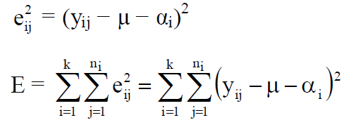
By this residual sum of squares E, we partially differentiate it with respect to
μ, and partially differentiating with respect to  and then equating these equations to 0, we get

Or

Or


So that-

Similarly-


Therefore-

And

And so on….
Test of hypothesis-
The hypothesis is-

 At least one population mean of a level of a factor is different from the
population means of other levels of the factor.
Or


Now, substituting these estimated values in the model given in equation (1),
the model becomes

And then-


Now substituting these values in equation (1) we get

Transporting by  to the left, and squaring both sides, and taking the sum over i
and j.


But 
since the sum of the deviations of the observations from
their mean is zero.
Therefore,


Where


So,

Degrees of freedom of various sum of squares-
Mean Sum of Squares
The sum of squares divided by its degrees of freedom is called the Mean Sum of Squares (MSS). Therefore,
MSS due to treatment (MSST) = SST/df = SST/ (k−1).
MSS due to error (MSSE) = SSE/df = SSE/ (N−k).
ANOVA table for one-way classification-
Source of variation | degrees of freedom (df) | Sum of squares (SS) | Mean sum of squares (MSS) | Variance ratio F |
Treatments | K – 1 |
| MSST = SST/(k-1) | F = MSST/MSSE With {(k-1), (N-k)} degrees of freedom |
Error | N – k |
| MSSE = SSE/(N – k) |
|
total | N – 1 |
|
|
|
Example: An investigator is interested to know the quality of certain electronic products in four different shops.
He takes 5, 6, 7, 6 products, and gives them a score out of 10 as given in the table-
Shop-1 | 8 6 7 5 9 |
Shop-2 | 6 4 6 5 6 7 |
Shop-3 | 6 5 5 6 7 8 5 |
Shop-4 | 5 6 6 7 6 7 |
Sol
If  denote the average score of electronic products of 4 shops then-
Null hypothesis-

Alternative hypothesis-

S. no. |
|
|
|
|
|
|
|
|
1 | 8 | 6 | 6 | 5 | 64 | 36 | 36 | 25 |
2 | 6 | 4 | 5 | 6 | 36 | 16 | 25 | 36 |
3 | 7 | 6 | 5 | 6 | 49 | 36 | 25 | 36 |
4 | 5 | 5 | 6 | 7 | 25 | 25 | 36 | 49 |
5 | 9 | 6 | 7 | 6 | 81 | 36 | 49 | 36 |
6 |
| 7 | 8 | 7 |
| 49 | 64 | 49 |
7 |
|
| 5 |
|
|
| 25 |
|
Total | 35 | 34 | 42 | 37 | 255 | 198 | 260 | 231 |
Total = 148
Correction factor = 
The raw sum of squares (RSS) =

Total sum of squares (TSS) = RSS – CF = 944 – 912.6667 = 31.3333
Sum of squares due to treatment (SST)-


Sum of squares due to error (SSE) = TSS – SST = 31.3333 – 5.1667 = 26.1666
Now-


ANOVA TABLE
Sources of variation | Df | SS | MSS | F |
Between shops | 3 | 5.1667 | 1.7222 | F = 1.7222 / 1.3083 = 1.3164 |
Within shops | 20 | 26.1666 | 1.3083 |
|
Here calculated F = 1.3164
Tabulated F at 5% level of significance with (3, 20) degree of freedom is 3.10.
Conclusion: Since Calculated F < Tabulated F, so we may accept H0, and conclude that the quality of shops does not differ significantly.
Question:
The following figures relate to production in kg. of three varieties P, Q, R of wheat shown in 12 plots
P 14 16 18
Q 14 13 15 22
R 18 16 19 15 20
Is there any significant difference in the production of these varieties?
Sol.
The null hypothesis is-

And the alternative hypothesis is-

Grand total = 14+16+18+14+13+15+22+18+16+19+19+20 = 204
N = Total number of observations = 12
Correction factor-

The raw sum of squares (RSS) =

Total sum of squares (TSS) = RSS – CF = 3552 – 3468 = 84
Sum of squares due to treatment (SST)-


Sum of squares due to error (SSE) = TSS – SST = 84 – 16.8 = 67.2
Now-


So that-

Sources of variation | Df | SS | MSS | F |
Between varities | 2 | 16.8 | 8.4 | F = 8.4/7.46 = 1.12 |
Due to error | 12 | 67.20 | 7.467 |
|
Total | 14 | 84 |
|
|
For  the tabulated value of F at 5% level significance is 4.261. Since the calculated value F is less than the table value of F, we accept the null hypotheses and conclude that there is no significant difference in their mean productivity of three varieties P, Q, and R.
“Statistical quality control is defined as the technique of applying statistical methods based on the theory of probability, and sampling to establish a quality standard, and to maintain it most economically”
The element of SQC-
Sample Inspection-
We know that the complete enumeration is not affordable every time, and it is could be very expensive, and time-consuming. 100% inspection is not practicable. Therefore SQC is based on sampling inspection. In the sampling inspection method, some items or units (called a sample) are randomly selected from the process, and then each, and every unit of the sample is inspected
Use of statistical techniques-
Statistical tools such as random sampling, mean, range, standard deviation, mean deviation, standard error, and concepts such as probability, binomial distribution, Poisson distribution, normal distribution, etc., are used in SQC. Since quality control method involves extensive use of statistics, it is termed as Statistical Quality Control
Decision making-
With the help of SQC, we decide whether the quality of the product or the process of manufacturing/producing goods is under control or not.
Note- the techniques of SQC are divided into two categories-
First- statistical process control (SPC)
Second- product control
Statistical process control-
A process is a series of operations or actions that transforms input to output. Statistical process control is a technique used for understanding, and monitoring the process by collecting data on quality characteristics periodically from the process, analyzing them, and taking suitable actions whenever there is a difference between actual quality, and the specifications or standard.
The statistical process control technology is widely used in almost all manufacturing processes for achieving process stability and making continuous improvements in product quality.
Tools we use in SPC-
Product control-
Product control means to control the products in such a way that these are free from defects and conform to their specifications.
Initially, product control was done by 100% inspection, which means that each, and every unit produced or received from the outside suppliers was inspected.
This type of inspection has the advantage of giving complete assurance that all defective units have been eliminated from the inspected lot. However, it is time-consuming and costly.
Sampling inspection or acceptance sampling was developed as an alternative to
100% inspection
Acceptance sampling is a technique in which a small part or fraction of items/units is selected randomly from a lot, and the selected items/units are inspected to decide whether the lot should be accepted or rejected based on the information obtained from sample inspection
Control charts-
Definition-
A control chart is a two-dimensional graphical display of a quality characteristic that has been measured or computed in terms of mean or another statistic from samples and plotted against the sample number or time at which the sample is taken from the process.
The concept of a control chart is based on the theory of sampling, and probability.
In a control chart, a sample statistic of a quality characteristic such as mean, range, the proportion of defective units, etc. is taken along the Y-axis, and the sample number or time is taken along the X-axis. A control chart consists of three horizontal lines, which are described below-
1. Centre Line (CL) – The centre line of a control chart represents the value which can have three different interpretations depending on the available data. First, it can be the average value of the quality characteristic or the average of the plotted points. Second, it can be a standard or reference value, based on representative prior data. Third, it can be the population parameter if that value is known. The centre line is usually represented by a solid line.
2. Upper Control Line – The upper control line represents the upper value of the variation in the quality characteristic. So this line is called the upper control limit (UCL). Usually, the UCL is shown by a dotted line.
3. Lower Control Line – The lower control line represents the lower value of the variation in the quality characteristic. So this line is called the lower control limit (LCL). Usually, the LCL is shown by a dotted line.
The UCL and LCL also have three interpretations depending on the available data same as the centre line. These limits are obtained using the concept of 3σ limits.
If all sample points lie on or in between the upper, and lower control limits, the control chart shows that the process is under statistical control. No assignable cause is present in the process. However, if one or more sample points lie outside the control limits, the control chart alarms indicate that the process is not under statistical control. Some assignable causes are present in the process, it is necessary to investigate the assignable causes, and take corrective action to eliminate them to bring the process under statistical control.
3σ limits-
The quality characteristic can be described by a probability distribution or a frequency distribution. In most situations, a quality characteristic follows a normal distribution or can be approximated by a normal distribution.
As we know that the probability that a normally distributed random variable (X) lies between 
 is 0.9973 where
  , and
, and  are the mean, and the standard deviation of the random variable (X). Thus

So the probability that the random variable X lies outside the limits  is
is
1– 0.9973 = 0.0027, which is very small. It means that if we consider 100 samples, most probably 0.27 of these may fall outside the  limits. So if an observation falls outside the
  limits in 100 observations, it is logical to suspect that something might have gone wrong. Therefore, the control limits on a control chart are set up by using
  limits. The UCL, and LCL of a control chart are called 3σ limits of the chart
Control charts pattern-
Their pattern is classified into two categories-
1. Natural patterns of variation, and
2. Unnatural patterns of variation.
Natural Patterns of Variation-
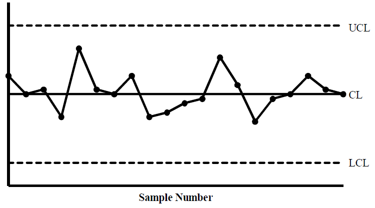
Most observations tend to concentrate near the centre (mean) of the distribution, and very few points lie near the tails Since the normal distribution is symmetrical about its mean (μ), i.e., the centre line is at μ, we expect that half the points will lie above the centre line and half below it. We also know that for the normal distribution-

This means that 99.73% of observations lie between the 3 limits. So of a total of
100 observations, 99.73 observations will lie inside the 3 limits, and only
0.27 observations may lie outside the 3 limits.
Unnatural Patterns of Variation-
There are 15 types of unnatural patterns in control charts.
We will study here some important types of unnatural patterns-
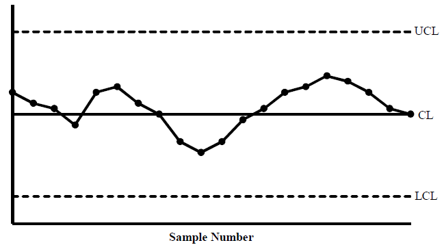
Cycles-
When consecutive points exhibit a cyclic pattern, it is also an indication that assignable causes are present in the process which affect it periodically
Causes of the cyclic pattern are:
i) Rotation of operators,
ii) Periodic changes in temperature, and humidity,
iii) Periodicity in the mechanical or chemical properties of the material,
iv) Seasonal variation of incoming component
Shifts-
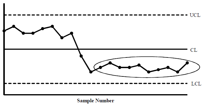
When a series of consecutive points fall above or below the centre line of the chart, it can be assumed that a shift in the process has taken place. This indicates the presence of some assignable causes
Causes of shift pattern are:
i) Change in material,
ii) Change in machine setting,
iii) Change in operator, inspector, inspection equipment
Erratic Fluctuations-
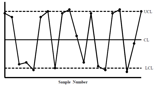
When the sample points of the control chart tend to fall near or slightly outside the control limits with relatively few points near the centre line. This indicates the presence of some assignable causes. The causes for erratic
fluctuations are slightly difficult to identify. These may be due to different
causes acting at different times in the process.
Causes of erratic fluctuations are:
i) Different types of materials being processed,
ii) Change in operator, machine, inspection, equipment,
iii) Frequent adjustment of machine
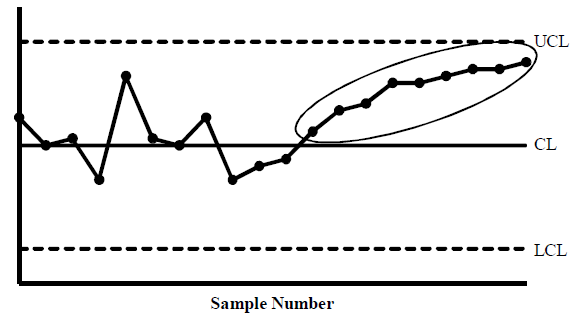
Trend-
If consecutive points on the control chart tend to move upward or downward. it can be assumed that the process indicates a trend. If proper care or corrective action is not taken, the process may go out-of-control.
Causes of trend pattern are:
i) Tool or die wear,
ii) Gradual change in temperature or humidity,
iii) Gradual wearing of operating machine parts,
iv) Gradual deterioration of equipment
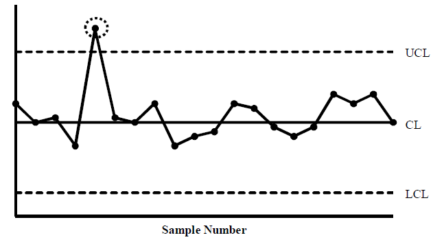
Extreme Variation-
If one or more samples point is significantly different from the other points, and lie outside the control limits of the control chart. there is an extreme variation in the chart. Some assignable causes are present in the process, and corrective action is necessary to bring the process under control.
Causes of extreme variation are:
i) Error in measurement, recording, and calculations,
ii) Wrong setting, and defective machine tools or erroneous use,
iii) Power failures for short time,
iv) Use of a new tool, failure of the component at the time of the test.
A sample point falling outside the control limits is a clear indication of the presence of assignable causes. There are other situations wherein the pattern of sample points on the chart indicates the presence of assignable causes, although all points may lie within the control limits
Control charts for variables (X, and R charts) –
In quality control, the term variable means the quality characteristic which can be measured, e.g., the diameter of ball bearings, length of refills, weight of cricket balls, etc. The control charts based on measurements of quality characteristics are called control charts for variables.
The most useful control charts are-
Now we will discuss them-
Control charts for mean (
If we want to control the process mean, in any production process, we use the control chart for the mean. With the help of the  -chart we monitor the variation in the mean of the samples that have been drawn from time to time from the process. We plot the sample means instead of individual measurements on the control chart because sample means are calculated from n individuals, and give additional information. The
  -chart is more sensitive than the individual chart for detecting the changes in the process mean.
Step by step method to construct the 
Step-1: We select the measurable quality characteristic for which the  -chart has to be constructed.
Step-2:
Then we decide the subgroup/sample size. Generally, four or five items are selected in a sample, and twenty to twenty-five samples are collected for the chart.
Step-3: After deciding the size of the sample, and the number of samples, we select sample units/items randomly from the process so that each unit/item has an equal chance of being selected.
Step-4: We measure the quality characteristic decided in Step 1 for each selected item/unit in each sample. Measurement errors may be due to many reasons. These may be due to many reasons.
These may be due to:
i) use of the faulty machine,
ii) different methods of taking measurements,
iii) inept use of instruments by unskilled or inexperienced work
force, etc.
Therefore, care should be taken that measurements are made by experts, using standard instruments.
Step-5: Calculate the sample mean for each sample.
Suppose we measure the quality characteristic, say, X for each unit/item of the sample.
Step-6: Set the control limits
To find out whether the process is under statistical control or out-of-control, we set up the control limits. The 3σ control limits for the  -chart is given by
Centre line = E(
Lower control limit = E(
Upper control limit = E(
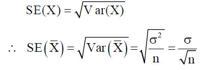
Where E( are the mean and the standard error of the sampling distribution of
 .
.
For getting the control limits of the  -chart we need the sampling distribution of the sample mean.
We know that  is a sample size drawn from a normal population with mean
The sample mean with mean  is normally distributed with
  .
.


We also know that-

Then the centre line, and control limits for the X-chart are given
as follows:
Centre line = E( =
= 
Lower control limit = 
Upper control limit = E( =
= 
Or
Lower control limit =
Upper control limit =
Where A = 
A is constant and depends on the size of the sample.
It has been tabulated for various sample sizes.
If values of μ and σ are not known. Therefore, these are estimated from the samples, which are taken when the process is thought to be under statistical control. We use their best possible estimates. the best estimators of the population mean (μ) and population standard deviation (σ) of the normal population are the sample mean, and sample standard deviation, respectively. So in this case, the best estimator of the process mean (μ) is the grand mean ( ), that is, the mean of all sample means given by

To calculate the grand mean, we first calculate the mean of each
Sample
Then we calculate the grand mean from the Equation.
Now, we need the best estimate of the unknown standard deviation σ.
It can either be estimated by sample range (R) or sample standard deviation (S). So we have two cases-
Case I: When the standard deviation is estimated by the sample range R.
In this case, the standard deviation σ is estimated as follows-

Where  represents the mean of all sample ranges given by-

Here  is the sample range, and is given by

And  is a constant, and depends on the size of the sample.
The control limits for the X-chart when μ is estimated by  and σ is estimated by
  are given by:
Centre line =  =
= 
Lower control limit =  =
= 
Or

Upper control limit =  =
= 
OR

When the standard deviation is estimated by the sample standard deviation.
In this case, the standard deviation σ is estimated as follows:


Here  is the sample standard deviation given by-

Therefore, the control limits for the  -chart when μ is estimated by
  and σ is estimated by S are given by-
Centre line =  =
= 
Lower control limit =  =
= 
Or

Upper control limit =  =
= 
OR

Step-7: Construct the X-chart
After setting the centre line, and control limits
It means that we take the sample number on the X-axis (horizontal scale), and the sample mean (X) on the Y-axis (vertical scale). We plot the value of the sample mean
for each sample against the sample number, and then join the consecutive sample points by line segments.
Step-8: Interpret the result
If all sample points on the plot lie on or in between upper, and lower control limits, the process is under statistical control. In this situation, only chance causes are present in the process. If one or more points lie outside the control limits the control chart alarms that the process is not under statistical control.
Range chart-
If  is a random sample of size n taken from a normal population with mean μ, and variance σ2, the mean, and variance of the sampling distribution of range are given as follows:-

And

 , and
, and  are constants, and depend on the size of the sample.
We know that-

And

Control limits are-
Central line- 
Lower control limit- E(R) – 3SE(R)
Upper control limit- E(R) + 3SE(R)
p-chart
Contol limits for p-chart-
CL = P
UCL = 
LCL = 
np- chart-
The np-chart is an adaptation of the basic p-chart. The purpose of this chart is to provide a better understanding of the operator who may understand an actual number of defective items easily rather than the proportion of defective. However, there is one drawback of the np-chart: It is used only for equal sample size because the number of defectives cannot be compared for variable sample size
Control limits for np-chart-
CL = nP
UCL = n
LCL = n
References
1. Erwin Kreyszig, Advanced Engineering Mathematics, 9thEdition, John Wiley & Sons, 2006.
2. N.P. Bali, and Manish Goyal, A textbook of Engineering Mathematics, Laxmi Publications.
3. P. G. Hoel, S. C. Port, and C. J. Stone, Introduction to Probability Theory, Universal Book Stall.
4. S. Ross, A First Course in Probability, 6th Ed., Pearson Education India,2002.


