UNIT 1
Two-dimensional force systems and Friction
Two-dimensional force systems:
When a single agency is acting on the body then it is known as force. But when numbers of forces are acting on the body simultaneously, then it is known “System of force”.
Types of Force System
1. Co-planer Forces
2. Non-Co-planer Forces
3. Co-linear Forces
4. Non-Co-linear Forces
5. Concurrent Forces
6. Non-Concurrent Forces
7. Parallel Forces (Like & unlike)
8. Coplanar Concurrent Forces
9. Coplanar Non-Concurrent Forces
10. Non-Coplanar Concurrent Forces
11. Non-Coplanar Non-Concurrent Forces
1. Co – planer Force System / Forces:-
The forces whose line of action lies on the same plane are called Co-planer Forces.
The forces which are acting in the same plane are known as co-planer forces.
2. Non-Co-planer Force System / Forces:-
- Forces whose line of action does not lie in the same plane ( i.e. lie in different planes )
- Forces that are acting in the different planes known as non-co-planer forces (system).
3. Co-linear force system / Forces:-
- The forces whose line of action lies on the same line are called co-linear forces.
- The forces which are acting along the same straight line are called co-linear forces.
4. Non – Collinear Forces/force system:-
- The forces which are not acting along the same straight line are known as non-co-linear forces.
- The forces whose line of action doesn’t lie on the same line.
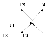
5. Concurrent forces/Force system:-
- The forces whose line of action meets at one common point are called concurrent forces.
- The forces which are passing through a common point are concurrent forces.
- The forces which meet at one point are concurrent forces.
6. Non-Concurrent force system/forces:-
- The forces which are not passing through common point OR
- The forces whose line of action does not meet at common point OR
- The force which does not meet at one point is called as non-concurrent forces.
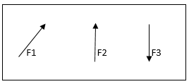
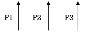
7. Parallel Forces / Force system:-
The forces whose lines of action are parallel to each other are called parallel forces.
a) Like parallel Forces:-
The forces whose lines of actions are parallel to each other and having the same direction are called Like parallel forces.
Forces that are parallel to each other & acting in the same direction are called as Like parallel forces.
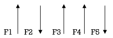
b. Unlike parallel Forces:-
The forces which are parallel to each other but having different directions or The forces which are parallel to each other & acting in opposite direction are called as unlike parallel forces.
8. Coplanar concurrent forces:-
The forces which meet at one point & their lines of action also lie on the same plane are called a coplanar concurrent force system.
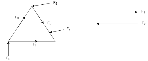
9. Coplanar non-concurrent forces:-
The forces which do not meet at one point but their line of action lies on the same plane are known as a coplanar non-concurrent system of force.
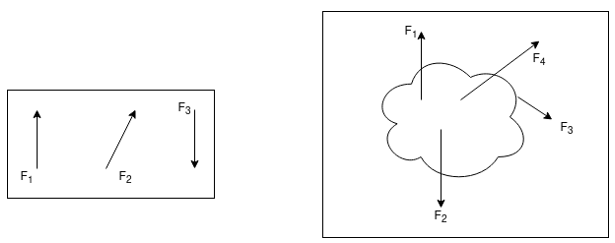
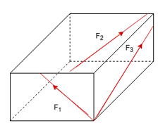
10. Non-Coplanar concurrent forces:-
The forces which meet at one point but their line of action do not lie on the same plane are known as non-coplanar concurrent forces.
11. non-coplanar non-concurrent forces:-
Their forces that do not meet at one point & their lines of actions do not lie on the same plane are called non - coplanar non-concurrent forces.
Newton’s first law states that, if a body is at rest or moving at a constant speed in a straight line, it will remain at rest or keep moving in a straight line at constant speed unless it is acted upon by a force. This postulate is known as the law of inertia. The law of inertia was first formulated by Galileo Galilei for horizontal motion on Earth and was later generalized by René Descartes. Before Galileo, it had been thought that all horizontal motion required a direct cause, but Galileo deduced from his experiments that a body in motion would remain in motion unless a force (such as friction) caused it to come to rest.
Newton’s second law is a quantitative description of the changes that a force can produce on the motion of a body. It states that the time rate of change of the momentum of a body is equal in both magnitude and direction to the force imposed on it. The momentum of a body is equal to the product of its mass and its velocity. Momentum, like velocity, is a vector quantity, having both magnitude and direction. A force applied to a body can change the magnitude of the momentum, or its direction, or both. Newton’s second law is one of the most important in all of physics. For a body whose mass m is constant, it can be written in the form F = ma, where F (force) and a (acceleration) are both vector quantities. If a body has a net force acting on it, it is accelerated in accordance with the equation. Conversely, if a body is not accelerated, there is no net force acting on it.
Newton’s third law states that when two bodies interact, they apply forces to one another that are equal in magnitude and opposite in direction. The third law is also known as the law of action and reaction. This law is important in analyzing problems of static equilibrium, where all forces are balanced, but it also applies to bodies in uniform or accelerated motion. The forces it describes are real ones, not mere bookkeeping devices. For example, a book resting on a table applies a downward force equal to its weight on the table. According to the third law, the table applies an equal and opposite force to the book. This force occurs because the weight of the book causes the table to deform slightly so that it pushes back on the book like a coiled spring.
The state of the rigid body will not change if the force acting on a body is replaced by another force of the same magnitude & direction acting anywhere on the body along the line of action of the replaced force. The value of force will not change along the Line of action of force within the body.
Parallel forces can be in the same or in opposite directions. The sign of the direction can be chosen arbitrarily, meaning, taking one direction as positive makes the opposite direction negative. The complete definition of the resultant is according to its magnitude, direction, and line of action.
When many forces are acting, the overall effect can be considered in a single force. This single force is called resultant force and the given individual forces are called component forces.
Methods for the resultant force
Though there are many methods for finding out the resultant force of a number of given forces, yet the following are important from the subject point of view:
2. Method of resolution.
The analytical method includes the Parallelogram law of Vectors which is described as “If two forces, acting simultaneously on a particle, be shown by two sides of a parallelogram, then the resultant will be the diagonal between these sides of a parallelogram.”
Mathematically, resultant force,

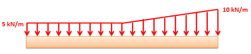
Where R is the resultant force, A and B are component vectors and  is the angle between the two vectors, as shown below.
For finding the direction of resultant vector, we need to find the angle between A and R i.e.  .
.
The resultant of this force system is either a single force or a couple.

The resultant is a couple when the resultant of all but one of the forces of the system and the remaining force form a couple. To determine the resultant analytically, each force is resolved into rectangular components in the x and y directions.
1When the algebraic sum of the components in either the x or y direction, or both, is different from zero, the resultant is a force, and its magnitude can be determined from the following equations:
Rx=∑Fx
RY=∑FY
R=√ (RX2+RY2)
Tan-1Θx=RY/RX
The location of a point on the action line of the resultant is determined by the principle of moments.
𝑅𝑞 = ∑𝑀𝑂
Where q is the perpendicular distance from the moment axis through o to the resultant force R. The direction from O to R is determined from the sense of R and ∑ 𝑀𝑂
2. When the algebraic sum of the components of the forces is zero in two different directions, the resultant cannot be a single force but can be a couple in the plane of the forces. The magnitude of the moment of the couple and its sense of rotation can be determined as the algebraic sum of the moments of the forces of the system with respect to any point in the plane.
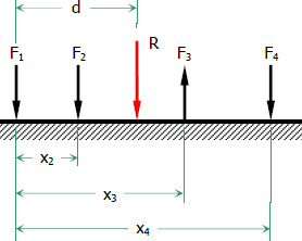
Note:- For the special case of a parallel coplanar force system with the x-axis parallel to the forces R of the system y = 0 and the resultant if a force is parallel to the x-axis
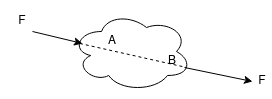
Distributed force is any force where the point of application of the force is an area or a volume. This means that the "point of application" is not a point at all. Though distributed forces are more difficult to analyze than point forces, distributed forces are quite common in real-world systems so it is important to understand how to model them.
Distributed forces can be broken down into surface forces and body forces. Surface forces are distributed forces where the point of application is an area (a surface on the body). Body forces are forces where the point of application is a volume (the force is exerted on all molecules throughout the body). Below are some examples of surface and body forces.
Distributed forces are represented as a field of vectors. This is drawn as a number of discrete vectors along a line, over a surface, or over a volume, that is connected with a line or a surface as shown below.
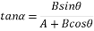
This is a representation of a surface force in a 2D problem (A force distributed over a line). The magnitude is given in units of force per unit distance.

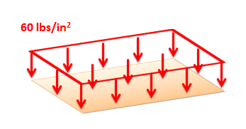
This is a representation of a surface force in a 3D problem (a force distributed over an area). The magnitude is given in units of force per unit area (also called a pressure).
Though these representations show a discrete number of individual vectors, there is a magnitude and direction at all points along the line, surface, or body. The individual vectors represent a sampling of these magnitudes and directions.
It is also important to realize that the magnitudes of distributed forces are given in force per unit distance, area, or volume. We must integrate the distributed force over its entire range to convert the force into the usual units of force.
For analysis purposes in statics and dynamics, we will usually substitute in a single point force that is statically equivalent to the distributed force in the problem. This single point force is called the equivalent point load and it will cause the same accelerations or reaction forces as the distributed force while simplifying the math. In the strength of materials context where the bodies are not rigid, this substitution will not work however as the distributed forces will not cause the same deformations and stresses as the point force.
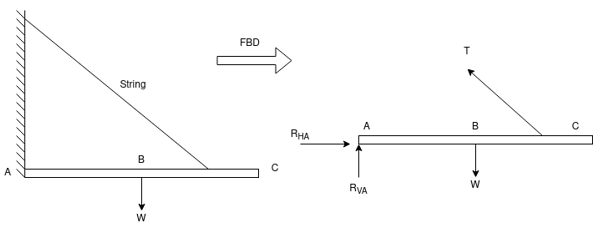
If a body is shown with all external forces acting on it so that the body is in equilibrium, such a diagram is called a free body diagram.
To draw the free body diagram, we have to remove all the restrictions like wall, floor, hinge, any other support and replace them by reactions which these support extents on the body.
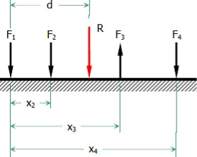
Ex – 1) Draw FBD of a bar supported and loaded as shown below.
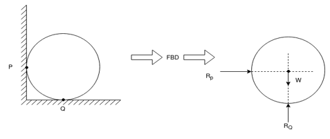
2) Draw FBD of sphere supported as shown below.

A free-body diagram is a sketch of an object of interest with all the surrounding objects stripped away and all of the forces acting on the body shown. The drawing of a free-body diagram is an important step in the solving of mechanics problems since it helps to visualize all the forces acting on a single object. The net external force acting on the object must be obtained in order to apply Newton's Second Law to the motion of the object.
A free-body diagram or isolated-body diagram is useful in problems involving the equilibrium of forces.
Free-body diagrams are useful for setting up standard mechanics problems.

Condition for Equilibrium: R = 0 {  }
}
∑M = 0
Equilibrium of the body subjected to two forces
P=Q, the body is in equilibrium P=Q, but the body is not in equilibrium
If an object is subjected to forces acting at two points, then the body will be in equilibrium only when those two forces are equal & opposite.
Equilibrium equation.
• Apply the equations of equilibrium, Σ Fx = 0 and Σ Fy = 0.
• The forces are directed as positive for those along the positive axis and vice-versa.
• If the resultant comes out to be a negative value, it means that the direction needs to be reversed for that is already considered.
As we know, the sufficient case for stating equilibrium for a body under a combination of forces is Σ F = 0.
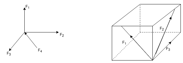
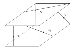
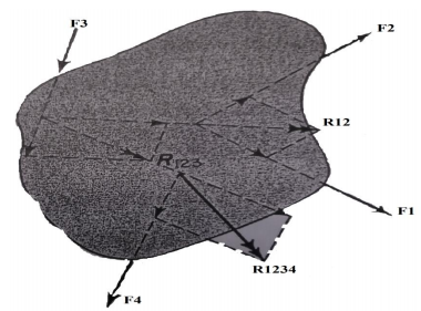
For any three-dimensional force system, as shown in Fig. below, we can resolve the forces into their respective i, j, k components, so that
Σ Fx i + Σ Fy j + Σ Fz k = 0
To satisfy this equation we require,
Σ Fx = 0
Σ Fy = 0
Σ Fz = 0
These three equations state that the algebraic sum of the components of all the forces acting on the particle along each of the coordinate axes must be zero. Using these equations mentioned we can solve for a maximum of three of the unknowns, shown by coordinate direction angles or magnitudes of forces shown on the particle’s free-body diagram.
For solving three-dimensional problems we can use the following procedure.
Free Body Diagram:
• In any orientation, establish x and y axes.
• Then mark all the known and unknown forces in the figure.
• Unknown forces are also assumed and plotted.
Equations of Equilibrium.
• Apply the equations of equilibrium, Σ Fx = 0, Σ Fy = 0 and Σ Fz = 0.
• Initially we can display as a Cartesian vector if it becomes to solve the problem regularly substitute these vectors into Σ F = 0 and then set the i, j, k components equal to zero.
• If the resultant comes out to be a negative value, it means that the direction needs to be reversed for that is already considered.
Application
A very basic concept when dealing with forces is the idea of equilibrium or balance. In general, an object can be acted on by several forces at the same time. A force is a vector quantity which means that it has both a magnitude (size) and a direction associated with it. If the size and direction of the forces acting on an object are exactly balanced, then there is no net force acting on the object and the object is said to be in equilibrium. Because there is no net force acting on an object in equilibrium, then from Newton's first law of motion, an object at rest will stay at rest, and an object in motion will stay in motion.
Let us start with the simplest example of two forces acting on an object. Then we will show examples of three forces acting on a glider, and four forces acting on a powered aircraft.
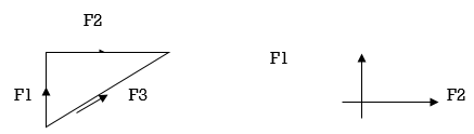
In Example 1 on the slide, we show a blue ball that is being pushed by two forces, labeled Force #1 F1 and Force #2 F2. Remember that forces are vector quantities and direction is important. Two forces with the same magnitude but different directions are not equal forces. In fact,
F1 = - F2
For the coordinate system shown with the letter X below the ball. If we sum up the forces acting on the ball, we obtain the force equation on the left:
F1 + F2 = F net = 0
Where F net is the net force acting on the ball. Because the net force is equal to zero, the forces in Example 1 are acting in equilibrium.
There is no net force acting on the ball in Example 1. Since the ball is initially at rest (velocity equals zero), the ball will remain at rest according to Newton's first law of motion. If the ball was traveling with a uniform velocity, it would continue traveling at the same velocity.
In Example 2, we have increased the magnitude of Force #1 so that it is much greater than Force #2. The forces are no longer in equilibrium. The force equation remains the same, but the net force is not equal to zero. The magnitude of the net force is given by:
F1 > - F2
F1 + F2 = F net
|F net| = |F1| - |F2|
Where the "| |" symbols indicate the magnitude of the quantity included between the ends. The direction of the net force would be in the positive X direction because F1 is greater than F2. According to Newton's second law of motion, the ball would begin to accelerate to the right. Because there is a net force in Example 2, the forces are not in equilibrium.
Friction:
Sliding Friction Formula
The equation for sliding force includes the coefficient of sliding friction times the normal force.
FS = μSFn
Where,
FS = force of sliding friction
μS = Coefficient of sliding friction
Fn = normal force
Factors affecting sliding friction
Examples of Sliding Friction
Sliding can occur between two objects of arbitrary shape whereas the rolling friction is the frictional force that is associated with the rotational movement. The rolling friction is usually less than the one associated with sliding kinetic friction. The values for the coefficient of rolling friction are quite less than that of sliding friction. It usually produces greater sound and thermal bi-products. For example- Movement of braking motor vehicle tires on a roadway.
A wedge is a piece of metal or wood that is usually of a triangular or trapezoidal in cross-section. It is used for either lifting loads through small vertical distances or used for slight adjustments in the position of a body i.e., for tightening fits or keys for shafts.
When lifting a heavy load the wedge is placed below the load and a horizontal force P is applied as shown in fig If the force P is just sufficient to lift the load, the wedge will move towards the left and the load will move up. When the wedge moves towards the left, the sliding of the surfaces AC and AB will take place. At the same time load moves up and sliding of the load takes place along GD. Thus for the wedge and load shown in Fig.3.41 sliding takes place along surface AB, AC, and DG. Hence there will be three normal reactions at AB, AC, and DG.
The problems on wedges are generally the problems of equilibrium on inclined planes. Therefore, these problems are solved by the equilibrium method or by applying Lami’s Theorem.

Equilibrium Method
In this method, the equilibrium of the load (or the body placed on the wedge) and the equilibrium of the wedge are considered.
Equilibrium of Wedge
Consider the equilibrium of the wedge. The forces acting on the wedge are shown in Fig. They are:
(i) The force P applied horizontally on face BC.
(ii) Reaction R1 on the face AC (The reaction R1 is the resultant of the normal reaction N1 on the rubbing face AB and force of friction on surface AC). The reaction R1 will be inclined at an angle θ1 (when θ1 is the angle of friction) with the normal.
(iii) Reaction R2 on the face AB (The reaction R2 is the resultant of normal reaction N2 on the rubbing face AB and force of friction on surface AB). The reaction R2 will be inclined at an angle Φ2 with the normal.
When the force P is applied on the wedge, the surface CA will be moving towards the left and hence the force of friction on this surface will be acting towards the right. Similarly, the force of friction on face AB will be acting from A to B.
References
1. Beer, F.P and Johnston Jr. E.R., “Vector Mechanics for Engineers (In SI Units): Statics and Dynamics”, 8th Edition, Tata McGraw-Hill Publishing company, New Delhi (2004).
2. Vela Murali, “Engineering Mechanics”, Oxford University Press (2010).
3. A Textbook of Engineering Mechanics, R.K. Bansal, Laxmi Publications.
4. Engineering Mechanics, R.S. Khurmi, S.Chand Publishing.
5. Meriam J.L. and Kraige L.G., “Engineering Mechanics- Statics - Volume 1, Dynamics- Volume 2”, Third Edition, John Wiley & Sons (1993).
6. Rajasekaran S and Sankarasubramanian G., “Engineering Mechanics Statics and Dynamics”, 3 rd Edition, Vikas Publishing House Pvt. Ltd., (2005).
7. Bhavikatti, S.S, and Rajashekarappa, K.G., “Engineering Mechanics”, New Age International (P) Limited Publishers, (1998).
8. Engineering mechanics by Irving H. Shames, Prentice-Hall.


