Unit - 2

Production Planning and control

2.1 Forecasting techniques – causal and time series models

Forecasting is critical in the creation of long-term strategies. Before investing in inputs, it is critical for organisations to determine what degree of activities they are intending.

Forecasting as defined by American Marketing Association is: "An estimate of sales in physical units (or monetary value) for ·a specified future period under proposed marketing plan or programme and under the assumed set of economic and other forces outside the organisation for which the forecast is made.

Prediction is the estimation of a future event based on subjective factors other than historical facts. A good subjective estimation for prediction is based on the manager's competence, experience, and judgement.

Today's forecaster has access to a wide range of forecasting methodologies of varying degrees of complexity. The availability of computer programmes has made the forecaster's job easier. Subjective methods are determined by individual judgments, while objective methods are determined after analysing quantitative data.

Forecasting methodologies are classified as follows:

• Judgemental techniques.
• Time Series methods.
• Causal methods (Econometric Forecasting)

The judgmental technique is a methodology that is based on human judgement.

This has been done for a long time. The other two approaches are newer and less well-known for analysing historical data, statistics are frequently used. The analyst seeks to establish cause and effect correlations in econometric forecasting between sales and some other sales-related parameter, such as the demand for, Cement is dependent on the construction industry's planned growth.

The goal of this strategy is to find a cause-and-effect link between changes in the product's sales level and a collection of explanatory variables. Regression and correlation analysis are used.

Time series analysis examines a product's historical demand pattern and projects or extrapolates that demand into the future. Time series analysis is a popular way for making predictions about the future based on what has happened in the past.

Time Series:

As a dependent variable, time is used as an independent variable, while time is used as a dependent variable.

The time series approaches do not investigate the elements that drive demand; instead, all of the factors that shape demand are bundled into one factor: time, and demand is expressed as a series of data with regard to time in this method.

The goal of time series analysis is to find the underlying demand pattern and extrapolate the future trend. The trend is determined using statistical approaches. There are four parts to a time series:

• Secular trend (T): A secular trend is the long-term tendency of data to increase or decrease. It is the long-term historical component of the time series that illustrates the business's general growth or decline over time.
• Cyclical Fluctuations (C) are the trend's oscillating patterns of growth or decrease. Some of the variation between the trend line and the data points is due to cyclical changes. Because the amount, timing, and pattern of cyclic fluctuations vary so significantly, the forecaster should be cognizant of the effect of cyclic variation.
• Seasonal Variations (S): These seasonal variations occur with considerable regularity over the course of a year and are annual. These variations are driven by meteorological circumstances, social practises, and holidays, such as the highest sales of paint during the Diwali Festival, the highest sales of umbrellas and raincoats during the monsoon, and the highest sales of warm clothing during the winter.
• Irregular Variations (R): These occur randomly and without any discernible pattern. These are random variations that can't be explained by trends, cyclic patterns, or seasonal changes. Natural disasters such as floods, draughts, earthquakes, and other natural calamities could be attributed to these factors.

The most used expression for a time series forecast is:

Y = TCSR

Where Y = Forecasted value

T = Secular trend

C = Cyclic variations

S = Seasonal variations

R = Irregular fluctuations

Least square method of forecasting (regression analysis):

This is the mathematical method of determining "the line of greatest fit between the dependent variable (typically demand) and an independent variable. Because the sum of the squares of the deviations of the various points from the line of best fit is minimum or least, this method is called the least square method. It specifies the line equation for which the sum of the squares of vertical distances between the actual and line values is the smallest.""

In a simple regression analysis, the relationship between the dependent variable y and some independent variable x can be represented by a straight line.

Where, b is the slope of the line & a is the y intercept

The values of the constants a and b are determined by the two simultaneous equations,

These two equations are called normal equations.

To compute the values of a and b,

• Calculate the deviation (x) for each period and the sum of deviations.
• Find the value of
• Find the value of
• Calculate the values of a and b
• Make the sum of deviations

Substituting the value of 0 in equations,

So,

Note:

• If the Time Series consists of odd number of years to make , the middle value of the time series is taken as the Origin.
• If the time series consists of even number of years, the midway period between two middle periods is taken as origin to make

Least square method when the sum of the deviations is not zero

For straight line,

Or, alternatively,

Causal methods (Econometric Forecasting)

Casual techniques attempt to discover the elements that influence demand fluctuation and to create a link between demand and these factors.

The analyst uses this strategy to try to find the factors that best explain the product's sales volume. This is known as econometric forecasting.

This method's goal is to establish a cause-and-effect relationship between changes in a product's sales level and a set of pertinent explanatory variables.

Some of the casual methods are,

• Regression and Correlation analysis.
• Input-output analysis.
• End use analysis.

Regression and Correlation:

The association between variables is established using regression analysis, which is a forecasting approach. A functional link between the two variables is established using historical data.

The degree of closeness of the relationship between two variables is determined via correlation analysis.

Any product's sales are influenced by external and internal factors in general. As a result, sales are a dependent variable that is influenced by one or more independent variables. The relationship between the independent and dependent variables is established using regression models (simple or complex).

Types of Correlation:

• Positive and Negative Correlation: Whether a link is positive (direct) or negative (indirect) is determined by the direction of fluctuation of variables (inverse or indirect). Positive correlation occurs when the value of one variable rises in tandem with the value of the other, indicating that both variables are moving in the same direction. If a rise (or decrease) in one variable causes an increase (or decrease) in another variable, the correlation is said to be negative.
• Simple and Multiple Correlation: When just two variables are involved, such as price and demand for a product, correlation is said to be simple. The correlation is considered to be multiple when more than two variables are evaluated at the same time. For example, consider the price, demand, and supply of a product.
• Linear and Non-linear Correlation

Co-efficient of correlation:

The degree of relationship is called correlation. It is a single figure which expresses the degree and direction of correlation is called co-efficient of correlation

Karl Pearson’s co-efficient of correlation:

The formula for calculation the co-efficient of correlation is given by

Where deviation of items of variable from its arithmetic mean

deviation of items of variable from its arithmetic mean

standard deviation of variable .

standard deviation of variable

The positive value of indicates +ve value of co-efficient of correlation.

The value of is between and .

The formula can be written in a simple way as

Where and .

The value of lies between and The value of one represents perfect correlation and value of zero indicates that there is no correlation between the two variables.

Regression Analysis

The regression co-efficient is the amount by which one variable varies in response to a change in another one.

The co-efficient of regression of on gives the value by which varies for a unit change, in . It is expressed as
Similarly, co-efficient of regression of on is expressed as
If is independent variable and is dependent variable, Then regression co-efficient of on is given by

If the deviations are taken from assumed means then the expression for regression of on is given as

If is independent variable and is dependent varia|ble Regression co-efficient of on is

Forecasting Error:

• Mean Absolute Deviation (MAD)

It is a measure of forecast error, and it measures the average forecast error without direction.

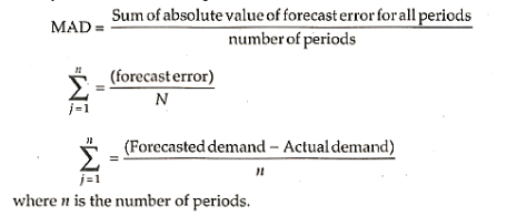
• BIAS

This measures the forecast error with regard to direction and shows any tendency to over forecast or under forecast.

This is also calculated as sum of forecast error for all periods divided by the total number of periods

2.2 Moving average

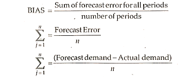
Because of seasonal and random variances, a company's previous sales statistics can exhibit fluctuations (high or low). Simple average of demand for prior periods will obscure the trend, which is irrelevant given the importance of the trend.

The Moving Average (MA) is made up of a series of arithmetic means determined from overlapping groupings of time series elements.

A moving average is a simple statistical tool for extrapolating and determining prior sales trends. This method calculates a rolling average for a set period of time using historical data. Because the data in this approach moves from period to period, it is called the moving average method. At the conclusion of each period, a fresh average is computed by adding the demand of the most recent period and removing the data of the previous period.

A simple moving average is calculated as follows:

Example:

For the time series of values for different periods,

The moving average for n periods,

The moving average period n should be properly chosen. The data will be distorted, and the trend will be misrepresented if the timeframe is chosen incorrectly. The smoothing effect is larger when the moving average period is longer.

The weightage of a three-month MA is one-third, and the weightage of a five-month MA is one-fifth. The smaller the effect of random variation and the higher the smoothing effect, the larger the value of n (moving average period). The value of n is determined by the rate at which the demand pattern changes. A high value of n is chosen if the demand pattern is stable.

A small value of n should be chosen if the pattern is not stable.

Centring of the Moving Average:

A three-period moving average is located against the second period, five months moving average is located against third month.

In general, n months moving average is located against,

Weighted Moving Average (WMA):

When a forecaster wishes to utilise a moving average, he or she doesn't always want all the periods to be equally weighted, as in the simple MA technique. Some organisations, however, use a weighted moving average to make their estimates.

In a three-month moving average, equal weight is given to the first, second, and third months in a simple MA. The organisation, on the other hand, wishes to give the third month more weight. And finally, the first month.

2.3 Exponential smoothing

One of the drawbacks of moving average forecasting is the time-consuming process of archiving data from earlier years. The current demand and the expected demand for the current month are all that is required for the exponential smoothing method. All the periods are given identical weightage in the simple moving average approach. Exponential smoothing is distinguished by the fact that it gives weight to all previous data and the weights are distributed in an exponential pattern.

The weights allocated to previous eras fall exponentially as demand for the most recent data increases. As a result, exponential forecasting ensures that the predictions provided by this method stay up with shifting business trends.

Exponential Smoothing Model,

Simple exponential smoothing model estimates the average forecast for the next period by using the actual and the forecasted demand for the previous period.

The basic advantage of this method over the moving average method is that one needs only two figures - one for the old forecast and another for the actual sales observation,

Expanding,

So,

Similarly,

So,

A general equation can be written as,

Were,

the starting forecast =, if an initial forecast cannot be made.

The importance of each of the previous requests is reduced by a factor of ten (1 - ). For a very large period value, the last term is negligible. If the demand pattern is smooth or constant, the value of an is minimal (0.05 to 0.1), whereas a big value of an is utilised for fluctuating demand.

2.4 Trend and seasonality

Trends are ignored by a simple exponential smoothing approach. A time series trend is a consistent increase or decrease in the series' average over time. When there is a considerable presence of a trend, the exponential smoothing strategy must be modified. There is a requirement to determine the trend estimate.

There are three steps to trend adjusted forecast.

1. Compute , the exponentially smoothed forecast for period 't' using the formula.

2. Compute the smoothed trend using the equation.

3. Calculate the forecast including the trend.

With trend adjusted approach, the estimates for both the average and the trend are smoothed and requires two smoothing constants. For each period, both average and trend are calculated,

As,

Were,

= exponentially smoothed average of series in period 't'.

= exponentially smoothed average of the trend in period

= smoothing parameter for the average.

= smoothing parameter for the trend.

= forecast for period t + 1

To make forecasts for period beyond the next period, multiply the trend estimate by the number of additional periods required in the forecast and add the results to the current average

Key takeaway

• Forecasting is a critical component of plan formulation. Before investing in inputs such as persons, machinery, and materials, it is critical for organisations to understand what level of activities they are intending.
• Forecasting is defined as "an estimate of sales in physical units (or monetary value) for a specified future period under a proposed marketing plan or programme and under the assumed set of economic and other forces outside the Organization for which the Forecast is made" by the American Marketing Association. As a result, forecasting is viewed as a projection based on historical facts. Forecasting is not a game of chance. It is a conclusion based on a significant amount of historical data.
• Forecasting is a crucial part of both strategic and operational planning. It creates a connection between planning and control. It is necessary for planning, scheduling, and managing the system in order to ensure that goods and services are produced effectively and efficiently.

• Forecasting is classed as long-term forecasting or short-term forecasting depending on the time period for which it is made. Short-term forecasting refers to forecasts that are made for periods of less than a year. Long-term projections are those that cover a period of more than one year (5 years or 10 years) in the future. Materials control, loading, scheduling, and budgeting are all aided by short-term projections. Product diversification, sales and advertising budgets, capacity planning, and investment planning all require long-term predictions.
• Time series approaches do not investigate the elements that drive demand; rather, all of the factors that shape demand are bundled into one factor—time—and demand is expressed as a series of data with respect to time in this method. The goal of time series analysis is to find the underlying demand pattern and extrapolate the future trend. The trend is determined using statistical approaches.
• Judgemental Techniques are widely employed in the business and industrial worlds. This is a subjective strategy that heavily relies on the person's previous experience and expertise.
• The mathematical method of establishing "the line of best fit between the dependent variable (typically demand) and an independent variable" is known as the least square method of forecasting (Regression Analysis). Because the total of the squares of the deviations of the various points from the line of best fit is minimum or least, this method is called the least square method. It specifies the line equation for which the sum of the squares of vertical distances between the actual and line values is the smallest.
• A moving average is a straightforward statistical tool for extrapolating and establishing prior sales trends. This method calculates a rolling average for a set period of time using historical data. Because the data in this approach moves from period to period, it is called the moving average method. At the conclusion of each period, a new average is computed by adding the demand from the most recent period and deleting the data from the previous period.
• The present demand and the expected demand for the current month are all that is required for the exponential smoothing method. All of the periods are given identical weightage in the simple moving average approach. Exponential smoothing is distinguished by the fact that it weights all previous data and the pattern is made up of exponentially weighted weights. The weights allocated to previous eras fall exponentially as demand for the most recent data increases. As a result, exponential forecasting ensures that the forecasts produced by this method stay up with shifting business trends.
• The causal forecasting method attempts to identify the elements that generate demand variation and to draw a link between demand and these factors. The analyst uses this strategy to try to find the factors that best explain the product's sales volume. This is known as econometric forecasting. The goal of this strategy is to find a cause-and-effect link between changes in the product's sales level and a collection of explanatory variables.
• Forecast Error refers to the numerical discrepancy between anticipated and actual demand. As far as feasible, the inaccuracy should be kept to a minimum. A good forecasting system should be simple to comprehend and use, with minimal forecast mistakes at the lowest possible cost, and stable in the sense that changes should be kept to a minimum.

Examples

Q.1.                     The following data gives the sales of the company for various years. Fit the straight line. Forecast the sales for the year 1998 and 1999.

Solution:

Year	Sale	Deviation
1	13		16
2	20		9
3	20		4
4	28		1
5	30	0	0	0
6	32	1	1	32
7	33	2	4	66
8	38	3	9	114
9	43	4	14	172

Now, substituting the values in the equations to get

The equation of the straight line of best fit is

(i) Sales for the year 1998

(ii) Sales for the year 1999

Q.2.                     A company manufacturing washing machines establishes a fact that there is a relationship between sale of washing machines and population of the city. The market research carried out reveals the following information.

Fit a linear regression equation and estimate the demand for washing machines for a city with a population of 45 million.

Solution:

Population	No. Of Washing sdemanded
5	28	25	140
7	40	49	280
15	65	225	975
22	80	484	1760
27	96	729	2592
36	130	1296	4680

To find the regression equation, the values of and are computed as follows:

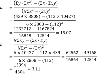
(i) The regression equation is

(ii) The demand for the washing machine when population of city is 45 million, i.e.,

Therefore, the number of washing machines demanded when is 155020 Nos. (Ans).

Q.3.                     Compute the load on the weaving machine centre using 5th moving average for the month of December 1996.Compute a weighted three months moving average for December 1996 where the weights are 0.5 for the latest month, 0.3 and 0.2 for the other months respectively.

Solution: Five months moving average forecast for Dec. 1996

(b) A three month weighted moving average forecast for Dec.

Q.4.                     The data given below represents sales figures of ABC company for the 12 months of the year 1996.

1. Compute 3 months moving average (ignoring decimal values) 2. Forecast the demand for the month of Jan. 1997 3. If the actual demand for the month of Jan. 1997 is 905 units. What should be the forecast for the month of Feb. 97.

Solution: (i) The 3 month moving average is shown in table below:

Month	Sales	Moving Total	Moving Average
Jan.	400
Feb.	490	1460	487
Mar.	570	1560	520
Apr.	500	1710	570
May	640	1820	607
June	680	2030	677
July	710	2190	730
Aug.	800	2330	777
Sept.	820	2530	844
Oct.	910	2590	864
Nov.	860	2720	907
Dec.	950

(ii) Forecast for the month of January is

(As the secular trend for Jan. 97 is not available, the forecast equals last moving average)

(iii) Forecast for Feb. 97

Q.5.                     The demand for the disposable plastic tubing for a general hospital is 300 units and 350 units for September and October respectively. Using 200 units as demand for September, compute the forecast for the month of November. Assume the value of a as 0.7.

Solution:

(i) Forecast ( can be written as,

In this case, Demand for September (300 units)

Forecast for October can be computed as,

(ii) Forecast for the month of November

Q.6.                     The following data relates the cost of production and sales prices.             

Establish the co-efficient of correlation between costs and prices.

Solution:

Costs X	Prices
203	225			2460	2520	2581
216	242			1340	1237	1142
223	250			876	764	666
239	271			185	65	23
248	275			21	4	1
253	277			0	0	1
279	295			697	507	369
301	318			2343	2042	1781
311	329			3411	3107	2830

Co-efficient of correlation between variable and is given by

i.e., close correlation between costs and prices.

2.5 Aggregate production planning

The process of establishing, assessing, and maintaining a preliminary, estimated timetable of an organization's total operations is known as aggregate planning. Targeted sales estimates, production levels, inventory levels, and customer backlogs are all part of the overall plan. This timetable is designed to meet the demand predicted at the lowest possible cost.

Critical factors before an aggregate planning process:

• Detailed information on the available manufacturing facilities and raw materials.
• A reasonable demand estimate for the medium term
• Budgeting for manufacturing costs, which covers raw materials, labour, inventory management, and so on.
• Organizational policies on labour management, quality management, and other issues.

Inputs required:

• A projection of total demand for the time period in question
• A review of all available options for managing capacity planning, such as subcontracting, outsourcing, and so on.
• -Present workforce operational state (number, skill set, etc.), inventory level, and production efficiency

Importance of aggregate planning:

• Achieving financial objectives by lowering all variable costs and increasing profit.
• Getting the most out of the limited production capacity
• Deliver customer delight by meeting demand and lowering client wait times.
• Cut back on inventory stocking costs.
• Capable of meeting scheduling objectives, resulting in a happy and pleased workforce

Objectives of aggregate planning:

• Maximize customer service
• Minimize inventory investment
• Minimize changes in workforce levels
• Minimize changes in production rates
• Maximize utilization of plant and equipment

Aggregate planning strategies:

Active Strategy:

• Attempts to manage demand variations by focusing on demand management.
• Uses pricing tactics and/or advertising and promotion.
• Develops counter-cyclical products
• Requests customers to back-order or advance-order.

Passive Strategy (reactive strategy):

• Focuses on supply and capacity management to handle demand fluctuations 
• Focuses on supply and capacity management to handle demand fluctuations
• Vary work force size by hiring or laying off 
• Vary labour and equipment utilisation through overtime or idle time 
• Build or draw from inventory 
• Subcontract production 
• Negotiate cooperative arrangements with other firms
• Allow backlogs, back orders, and/or stock-outs

Mixed strategy:

• Combines components of both an active and a passive (reactive) strategy.
• Most businesses will use a combination of the two.

There are three types of aggregate planning strategies available for organization to choose from. They are as follows,

Level Strategy:

Level strategy, as the name implies, aims to maintain a consistent production pace and labour level. To enhance or decrease production in anticipation of lower or higher consumer demand, the business needs a strong forecast demand. The advantage of a level plan is that it ensures a consistent workforce. Level strategy has a lot of disadvantages. Inventory should be increased, as well as backlogs. Capacity (number of employees, production schedules, etc.) Over the planning horizon, output rates, etc.) are kept constant. The goal of a level strategy is to find a middle ground. To create an overall plan that maintains a constant pace of production and/or a constant rate of output degree of employment

In order to meet changing client demand, the company must increase or decrease inventory levels in anticipation of higher or lower predicted demand. When demand is low, the company maintains a consistent staff and output rate. This permits the company to stockpile more goods than is currently required. As demand rises, the company is able to maintain a consistent production rate/level of employment while allowing the inventory excess to absorb the additional demand.

Another option is to employ a backlog or back-order system. A back-order is just a commitment to deliver the product at a later date, usually when capacity catches up with falling demand. In essence, a back-order is a mechanism for shifting demand from one period to another, preferably one with lower demand, to normalise demand requirements over time.

A level approach allows a company to keep its output constant while yet meeting demand. From the aspect of employee relations, this is ideal. Excess inventory expenses, subcontracting or overtime charges, and back-order costs, which are often the cost of expediting orders and the loss of consumer goodwill, are all negative outcomes of the level strategy.

Advantages:

• Stable output rates and workforce levels Produce as much as needed
• Zero inventory, no holding cost, no shortages
• Zero inventory is difficult to achieve because work hours may not be flexible
• Low inventory costs, high smoothing costs

Disadvantages:

• Greater inventory investment is required
• . (ii) Increased overtime and idle time
• Resource utilizations vary over time

Chase Strategy:

Chase strategy, as the name suggests, aims to dynamically match demand with output. Lower inventory levels and backlogs are advantages of the chasing strategy. Lower productivity, poor quality, and a depressed workforce are all disadvantages. Capacity (number of employees, production) Over the planning period, timetables, output rates, and so on) are altered to fulfil demand requirements horizon. In a chase approach, demand and capacity are matched period by period. This could result in a large number of employees being hired, fired, or laid off; insecure and disgruntled staff; increasing inventory carrying expenses; labour union issues; It also has irregular plant and equipment utilisation.

It also shows that the company is willing to be flexible. The main benefit of a chase strategy is that it allows inventory to be retained at the lowest level feasible, which can save a lot of money for some businesses. When it comes to aggregation planning, most companies that embrace the just-in-time production idea use a chase strategy. Most businesses find it beneficial to combine the level and chase strategies.

A combination strategy (also known as a hybrid or mixed strategy) can be utilised to better accomplish company goals and policies while also lowering expenses as compared to either of the pure techniques employed separately.

Advantages:

• Anticipation inventory is not required, and investment in inventory is low
• Labour utilization is kept high Produce a constant amount each period
• Stable workforce, no hiring/firing, no overtime,
• No subcontract
• Low smoothing costs, high inventory costs

Disadvantages:

• Expense of adjusting output rates and/ or workforce levels alienation of workforce

Hybrid Strategy:

Hybrid strategy, as the name implies, aims to strike a balance between level and chasing strategies. Two extreme methods are the chase and level strategies. Inventory costs are reduced with the chase approach, while smoothing costs are reduced with the level strategy. The purpose of optimization is to find a manufacturing strategy that reduces overall inventory and smoothing costs. Linear programming can be used to accomplish this.

Aggregate Planning Methods: Intuitive Methods

Intuitive methods use management intuition, experience, and rules-of-thumb, frequently accompanied by graphical and/ or spreadsheet analysis.

Advantage:

• Easy to use and explain

'Disadvantage:

• Many solutions are possible, most of which are not optimal

Matching Capacity and Demand:

Options to match Capacity:

• Pricing
• Promotion
• Back ordering
• New demand creation

Options which can be used to increase or decrease capacity to match current demand include:

• Hire/Lay off
• Overtime
• Part time or casual labour
• Inventory
• Subcontracting
• Cross training

Aggregate Planning Strategies:

• Vary the Workforce Size: Output is managed by hiring and firing personnel in response to changes in demand.
• Vary Working Hours: Maintain a consistent workforce, but provide idle time when demand is low and overtime (OT) when demand is high.
• Vary Inventory Levels: A big amount of inventory can be used to meet demand swings.
• Subcontract: Upward change in demand from low level. Subcontractors can be used to supply extra capacity to maintain consistent production rates.

Strategies to Meet Non-uniform Demand:

Aggregate planning guidelines:

• Determine the company's policy on controllable variables.
• Plan with the help of a good prediction.
• Include the appropriate capacity units in your planning.
• Maintain a consistent staff.
• Maintain inventory management as appropriate.
• Maintain flexibility in the face of change.
• Act in a regulated manner in response to demand.
• Review your plans on a frequent basis.

Key Takeaway

The process of establishing, assessing, and maintaining a preliminary, estimated timetable of an organization's total operations is known as aggregate planning. Targeted sales estimates, production levels, inventory levels, and customer backlogs are all part of the overall plan. This timetable is designed to meet the demand predicted at the lowest possible cost.

Aggregate planning is of the medium-term (rather than long- or short-term) variety. As a result, most aggregate plans are for three to eighteen months. Aggregate plans are used to lay the groundwork for future short-term planning, such as production scheduling, sequencing, and loading.

Active strategy, Passive strategy (reactive strategy), and Hybrid strategy are the three Aggregate Planning strategies.

Level strategy, as the name implies, aims to maintain a consistent production pace and labour level. In order to enhance or decrease production in anticipation of lower or higher consumer demand, the business needs a strong forecast demand.

The advantage of a level plan is that it ensures a consistent workforce.

High inventory and increased backlogs are disadvantages of level strategy. Over the planning horizon, capacities (workforce levels, production schedules, output rates, and so on) are kept constant. A level strategy aims to create an overall plan that maintains a constant pace of output and/or employment.

Strategy of Pursuit, Chase strategy, as the name suggests, aims to dynamically match demand with output. Lower inventory levels and backlogs are advantages of the chasing strategy. Lower productivity, poor quality, and a depressed workforce are all disadvantages. Over the planning horizon, capacities (workforce levels, production schedules, output rates, and so on) are changed to fit demand requirements. In a chase approach, demand and capacity are matched period by period.

Strategic alternatives for aggregate planning: the production system's variables are labour, materials, and capital. To produce a bigger volume of output, more labour effort is necessary.

As a result, the two relevant factors are employment and overtime usage. Materials aid in the control of output. Inventories, backordering, and item subcontracting are some of the options open to the company.

These controllable variables are pure solutions for accommodating demand changes and uncertainties in industrial activities. Several choices are available, including:

• Vary the size of the workforce: output is managed by hiring and firing personnel in response to demand fluctuations.

• Vary the hours worked: keep the staff consistent but allow idle time when demand is low and overtime when demand is high.

• Vary inventory levels: a big amount of inventory can be used to meet demand swings.

• Subcontract: demand has shifted upward from a low point. Subcontractors can be used to supply extra capacity to maintain consistent production rates.

One of the allocating capabilities (supply) to fulfil predicted (demand) requirements is the aggregate planning problem. It's possible to solve it using linear programming.

The problem can be solved by using a transportation technique.

2.6 Master production scheduling (MPS)

Aggregate planning is followed by master scheduling. It presents the overarching strategy in terms of distinct end products or models to which priority can be allocated. It's a good idea to plan ahead for material and capacity needs.

Functions of MPS:

The master production schedule (MPS) formally documents the production plan and turns it into material and capacity requirements. After then, the labour, material, and equipment requirements are evaluated.

• To convert aggregate plans into specific end items: An aggregate plan establishes the level of operations that attempts to match market needs with the company's material, labour, and equipment capabilities. This plan is translated into a particular number of end goods to be produced in a certain time period by master schedules.
• Compare and contrast alternative schedules: The master schedule is created by trial and error. To analyse the alternative schedules, a variety of computer simulation models are available.
• Create Material Requirements: This is the first step in the material requirement planning process (MRP).
• Create Capacity Requirements: MPS is used to create capacity requirements. As a result, master scheduling is a requirement for capacity planning.
• Facilitate Information Processing: The plant master schedule specifies when the delivery should be made by controlling the load on the plant. It works in conjunction with other management information systems such as marketing, finance, and human resources.
• Effective Capacity Utilization: The master schedule determines the load and utilisation requirements for machines and equipment by providing end item needs.

Time Intervals and Planning Horizon:

The type, volume, and component lead times of the items being produced determine the time interval employed in master scheduling. Normally, time periods of one week are employed. The master schedule's time horizon is also influenced by product attributes and lead times. Some master schedules include as little as a few weeks, while others encompass more than a year.

Master schedules often have firm and flexible portions.

Changes in master schedule affect lead times, work schedules, machine set-ups.

"Firm" portion will encompass the minimum lead-times necessary for components and cannot be changed.

Aggregate Plan
Month
No. Of Motors	30	45	50	30	60	30	30	40	40
Master Schedule
Month
Ac Motors (5 HP)	5	5	10	5	15	6	10		10
20 HP	10	7	10	5	10	4	5		20
D.C. Motor 20 HP	5	10	15	10	15	10		5	10
FHP Motors (1/2 HP)	10	23	15	10	20	10		35

A Master Production Schedule Example:

Months and then weeks are used to split the quarterly time chunks. Each product family's quantity to be produced in a quarter is divided by the number of weeks in that quarter. Based on the mix of those items in the current demand pattern and adjusted or existing inventory levels of each product, the total quantity of a product family to be made in a week is divided among individual product models in that family. Every week, MPS is examined to ensure that the correct mix of products is being generated, especially for the week that is about to enter the time fence.

2.7 Materials requirement planning (MRP) and MRP‐II

"Materials Requirement Planning (MRP) is a technique for determining the quantity and timing for the acquisition of dependent demand items needed to satisfy master production schedule requirements"

MRP Objectives:

• Inventory Reduction
• Reduction in Manufacturing & Delivery Lead times
• Realistic Delivery Commitments
• Increased Efficiency

Function Served by MRP

Inventory control, bill of material processing, and basic scheduling are all core operations of an MRP system. MRP assists businesses in maintaining low inventory levels. It's used to schedule manufacturing, purchasing, and delivery.

MRP can be used to track things purchased from outside vendors as well as sub-assemblies made in-house that are parts of larger, more complex items.

• Order Planning and Control: When and for what quantities of materials/components should orders be released.
• Priority Planning and Control: How does the estimated availability date for each component compare to the required date?
• Providing a foundation for forecasting capacity needs and formulating comprehensive business plans.

MRP Terminology:

• Dependent Demand: When the demand for one thing is influenced by the demand for another. The degree to which demand for one thing is linked to demand for another is known as demand dependence.
• MRP- A method for estimating the quantity and timing of demand items that are dependent on one another.
• Lot Size- The number of products needed to complete an order.
• Scheduling to produce or receive an adequate amount (Lot) of material in the time periods when it is required.
• Time Bucket- In MRP, the time period employed for planning purposes is referred to as a time bucket.
• Gross Requirements- The total amount of an item required at the conclusion of the period in order to satisfy the planned output levels.
• Net Requirements- The net quantity of an item that has to be purchased in order to meet the period's output schedule. Gross requirements minus scheduled receipts for the period minus monies available from the previous period is how it's determined.
• Requirements Explosion- The dismantling (explosion) of parent things into component portions that can be planned and scheduled individually.
• Scheduled Receipts- The amount of an item that will be received from suppliers in response to orders placed.
• Planned Order Receipts-The quantity of an item that is planned to be ordered and received at the start of the period in order to meet the period's net requirements. The purchase order has yet to be placed.
• Scheduled Order Release- The quantity of an item that is planned to be ordered or a plan (quantity and date) to begin the acquisition or manufacture of materials so that they arrive on time following the lead time offset.
• The supply time or number of time buckets between releasing an order and receiving the materials is referred to as the lead time offset.

Benefits and drawbacks of MRP:

Manufacturing companies can profit from MRP systems in a variety of ways. Helping production managers minimise inventory levels and associated carrying costs, track material requirements, determine the most cost-effective lot sizes for orders, compute quantities needed as safety stock, allocate production time among various products, and plan for future capacity needs are just a few of the main benefits.

MRP systems may potentially have a number of disadvantages. First and foremost, MRP relies on correct input data. If a small business does not keep proper inventory records or does not keep up with all essential changes in its bills of materials, it may have major issues with its MRP system's outputs. Missing parts, high order quantities, timetable delays, and missed delivery dates are all possible issues.

Another major disadvantage of MRP is that it can be complex, time-consuming, and expensive to adopt.

MRP System:

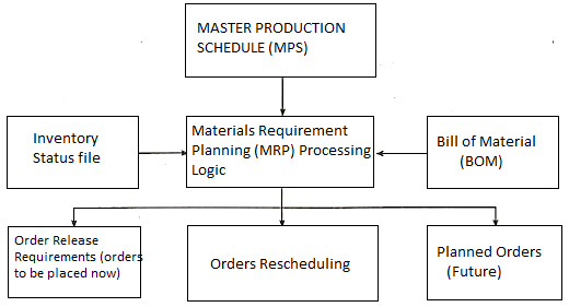
MRP Output:

TO MPS Planners'

• Simulation of proposed MPS
• Researching information for open orders (due to cancellation, delays, shortages)

To Purchasing and Production

• Changes to keep priorities valid.
• Order releases (Purchase and shop orders)
• Planned order releases

To capacity Requirements Planning

• Order release information for load profiles, delays, shortages

To Management

• Performance measurement of (vendors, cost, forecast accuracy)
• Exception reports (on due dates BOM file, etc.)

MRP Logic:

MANUFACTURING RESOURCE PLANNING (NRP-II):

Manufacturing Resource Planning II (MRP-II) is a comprehensive information system that synchronises all areas of a company's operations. By adopting a focal production plan and employing a single unified data base to plan and update activities in all systems, the MRP-II system coordinates sales, purchasing, manufacturing, finance, and engineering.

A manufacturing resource planning can be broken down into three sections:

• Product planning functions that take place at the top management level.
• Staff units are in charge of operations planning.
• Manufacturing line and staff managers oversee operations control.

Checkpoints between the three divisions offer input on the overall adequacy of resources, the completeness of resource commitments, and the quality of execution of the plans. Feedback based on these checks allows for a speedy response to changing conditions while still employing the most up-to-date operating data.

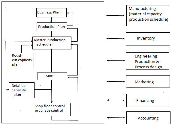
The method (as depicted in the diagram) entails creating a production plan from the business strategy in order to determine monthly production levels for each product line for the following five years. The production department is then expected to produce at the committed levels, the sales department to sell at these levels, and the finance department to guarantee that sufficient financial resources are available to support these levels. The production schedule is then guided by the production plan, which specifies the weekly amounts of individual goods to be built.

Then the available capacity is nearly adequate. If this is not the case, either the master schedule or the capacity are altered. This master schedule is then used in MRP to establish material requirements and production priority schedules. After then, a study of precise capacity requirements establishes whether capacity at each work centre is sufficient for scheduled time periods.

Then, to ensure that the master schedule is met, the execution and control activities are determined.

Key Takeaway

"Materials Requirement Planning (MRP) is a technique for determining the quantity and timing for the acquisition of dependent demand items needed to satisfy master production schedule requirements"

2.8 Routing

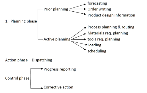
Routing may be defined as the process of determining how to get from point A to point B "Selection of suitable procedures to be followed by each component of the product as it is transferred from raw materials to completed goods. The path of the goods will also indicate the order in which actions should be performed throughout production."

In other words, routing is the process of determining the most efficient path to take from department to department and machine to machine till raw materials reach their ultimate shape.

Routing identifies the most efficient and cost-effective sequence of processes and ensures that it is strictly followed.

Routing is a crucial PPC function since it has a direct impact on the operation's "time" and "cost." Backtracking and extended journeys are examples of bad routing. This will cause the processing time to be extended needlessly. Furthermore, the cost of material handling will rise. Plant layout has an impact on routing. In fact, route and plant layout are inextricably linked. The routing in product layout is short and straightforward, whereas it is long and complex in process layout.

Routing Procedure:

1. Product analysis: the finished product is analysed and broken down into the number of components needed for the product.

2. Make and buy decision: This refers to whether all components will be created in-house or will be obtained from outside sources. The decision to make and buy is based on

• The workload in the plant already existing
• Availability of equipment’s
• Availability of labour
• Economy consideration

3. Needs for raw materials

A part list and bill of materials is created, which includes the name of the part, the number of materials specified, and the number of materials necessary, among other things.

4. A list of the processes that the raw materials will go through is provided.

5. The machines that will be used, as well as their capacities, are listed.

6. Each operation and subassembly's time requirements are listed.

7. The small size is also noted.

The information gathered this way is used to create master route sheets and operating charts. The master route sheets provide information on when different operations should begin and end to achieve the product and the requisite time.

The route sheet for the individual item or component is the next stage.

Route sheet:

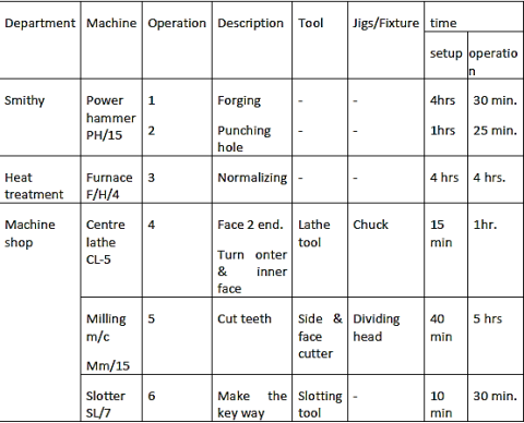
Only a small difference exists between the operation sheet and the route sheet. An operation sheet contains information such as operation descriptions, sequence, kind of machines, tools, jigs and fixtures required, setup and operation time, and so on. The route sheet, on the other hand, specifies the section (or department) and the specific machine on which the job is to be performed.

If the order is repeated, the operation sheet will remain the same, but the route sheet may need to be altered if specific machines are already engaged to fulfil the request.

Except for a few minor differences, these sheets contain nearly identical information and are thus commonly combined into a single page known as the operation and route sheet.

Advantages of Routing

1. Efficient use of available resources.

2. Reduction in manufacturing cost.

3. Improvement in quantity and quality of the o/p.

4. Provides the basis for scheduling and loading.

2.9 Scheduling and priority dispatching

Most of the other controls are built on the foundation of production control.

Control is defined as the act of forcing actions to follow a set of rules. "Production control is a management function that plans, directs, and controls an enterprise's material supply and processing activities so that specified products are produced by specified methods to meet an approved sales programme," according to Wikipedia. "These activities are carried out in such a way that the available labour, plant, and capital are used to the best advantage." Programming, ordering, and dispatching are the three layers of production control.

• Programming is the process of determining how many things will be produced.
• Ordering schedules the delivery of components from suppliers and departments in order to fulfil the program's deadlines.
• Dispatching looks at each department separately and plans the output from equipment and work centres required to complete the orders.

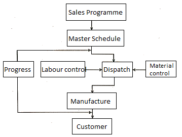
Loading and scheduling: A works order will be issued by the sales department, authorising the creation of a product or group of products. This order serves as the beginning point for all of the production control department's efforts related to product manufacturing. The master production schedule (MPS) is created, which includes identifying the dates by which important functions must be performed, as well as assessing labour and material requirements and availability. It is completed the loading of numerous work centres. Material control will receive a copy of the Master Schedule and will check material availability.

• Material control: The material control component of production control's function is to analyse the need for material and then take suitable activities (actions) to meet those needs.
• Dispatch and progress: A manufacturing process is started at a specific time that gathers all essential documents, confirms the availability of each of the production factors, and authorises the start of production activities through the issuance of authorising documents. The progress section will keep track of performance and ensure that the master schedule's requirements are met. Any deviations from this schedule are brought to the attention of those involved, and remedial action is taken to maintain the departure to a minimum.

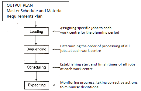
Loading, sequencing, and scheduling:

Output plans define when products are required, but they must be translated into operational terms before they can be implemented on the shop floor.

Loading:

When job orders are released, they are assigned to work centres, determining the amount of burden each work centre should carry for the given planned period. This task is known as loading. A load is the amount of work allotted to a machine or an operator, while capacity is the amount of output that can be produced in a reasonable amount of time.

• Loading is the study of relationship between load and capacity at work centres.
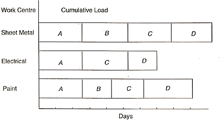
• Gantt Load Charts, Visual load profiles are helpful for evaluation of the current loading.

Gantt Chart:

It is the most important tool for both loading and scheduling. Henry L. Gantt, an American engineer, invented the chart, which consists of a simple rectangular grid separated by a series of parallel horizontal and vertical lines. The chart is divided into time units by vertical lines. According on the duty for which the chart is required, the scale units can be years, months, weeks, days, or hours. The chart is divided into portions by horizontal lines, which can represent work tasks or work centres. When it comes to presenting critical shop information, the Gantt chart has the benefits of simplicity and clarity. To account for new job assignments, the Gantt chart must be updated on a regular basis.

Example:

Visual Load Profiles

On a time, scale, it's a graph that compares workloads and capacities. The load in a manual scheduling system is made up of open orders (client orders that have not yet been filled) that have been assigned to a work centre.

Open orders and scheduled orders make up the load in computer-based scheduling systems (Prospective Orders from customers).

When there are overloads, some of the work will be sent to other work centres.

This can be accomplished in two ways.

• Lot splitting: In which a job order is split and only part of it is processed now and others are processed later.
• Operations splitting: Processing part of the job in one work centre and the rest at another.

Priority sequencing:

Which job should be done next when jobs compete for work centre capacity? All jobs in the queue are subject to priority sequence rules. When the job's work centre becomes available, the one with the highest priority is allocated. "Priority Sequencing" is a method of assigning priorities to waiting jobs to determine the order in which they will be completed.

Choosing criteria for sequencing:

• Set up cost.
• In process inventory.
• Idle times.
• Average time to complete jobs.
• Average number of jobs waiting in the queue.
• Average time the jobs are late.

Other factors represent both customer service and internal facility efficiency, such as set-up cost, inventory cost, and idle times.

Priority sequencing rules:

• First come, first served (FCFS): Gives the highest priority to the job in queue that arrives first in the production system.
• EDD (earliest due date): Gives top priority to the waiting job with the earliest due date.
• Shortest processing time (SPT): Prioritizes the waiting job with the shortest operating time at the work centre.
• Least slack (LS): Slack is computed as the difference between the amount of time left until the job is due and the amount of time it takes to complete it.
• Processing time is the longest (LPT).
• Favourite customer order (PCO).

Sequencing Problem:

The sequencing problem arises when it is necessary to determine the best order in which to conduct a number of jobs by a number of facilities according to a predetermined order in order to maximise output in terms of cost, time, or profit.

The production of finished goods from raw materials entails a series of procedures that must be completed in a specific order. Similar activities for many goods are frequently done at the same workstations, especially in intermittent or batch production. In such cases, selecting a preferred order for products travelling through a workstation is needed. When many workstations serve multiple products, the problem becomes more complicated. The minimum total processing time is the criterion in such a problem.

The general sequencing problem is stated as,

Processed in Machines one at a time,

The order of processing each job through the machines is given and also the time taken to process each job on each machine is known.

The problem is to determine the order of processing of n jobs so that the total elapsed time for all the jobs will be minimum. The general sequencing problem is to determine the optimal sequence from amongst sequences that minimises the total elapsed time.

Assumptions:

• No machine can process more than one job at a time.
• Processing times are independent of processing of jobs.
• Each job once started on one machine is continued till completion on it.
• Time involved in moving a job from one machine to another is negligibly small.

The satisfactory solutions are available for the following problems

      n jobs and 2 machines (Johnsons Algorithm)

Machines = A & B

Jobs is processed in the order A & B

Processing time of n Jobs =

Processing time on A =

Processing time on B =

The problem is to find the order in which the n jobs are to be processed to minimise the total elapsed time to complete all the n jobs.

Procedure:

• Step 1: Select the smallest processing time from the given list of processing times A1, A2 A„ and B1, B2 B„
• Step 2: If the minimum processing time is Ar (i.e., Job number r on Machine A), do the rth job first in the sequence. If the minimum processing time is B, (i.e., job numbers on Machine B, do the sth job last in the sequence.
• Step 3: After doing this step, (n-1) jobs are left to be sequenced. Repeat step (1) and step (2) till all the jobs are ordered.
• Step 4: Find the total processing time as per the sequence determined and determine idle time associated with machines.

• n jobs and 3 machines

Machines =

Jobs is processed in the order

• The smallest processing time on machine M1 largest processing time on machine M2.
• 2. The smallest processing time on machine M3 largest processing time on machine M2.

If either or both above stated conditions are satisfied, the given problem can be solved by Johnson's algorithm.

Procedure:

• Convert the three-machine problem into two machine problems by introducing two fictitious machines G and H.
  • 
  • 
• Once the problem is converted to n job .2 machine the sequence is determined using Johnson's algorithm for n Jobs and 2 machines.
• For the optimal sequence: determined, find out the minimum total elapsed time and idle times associated with machines.

Tie breaking Rules

• If there are equal smallest processing times one for each machine, place the job on machine 1, first in the sequence and one in machine 2 last in the sequence.
• If the equal smallest times are both for machine 1, select the job with lower processing time in machine 2 for placing first in the sequence.
• If the equal smallest times are both form Machine 2, select the one with lower processing time in machine 1, for placing last in the sequence.

• n jobs and m machines

Let there be n jobs which are to be processed through m machines M1, M2 M„ in the order Ml, M2 - Mne

Let Tii denote the time taken by jth job on the ith machine.

Procedure:

Step 1: Find (i) Min (Minimum time for the first machine)

(ii) Min (Minimum time on the last machine)

(iii) Maximum time on intermediate machines.

Max (,

(For j = 1,2,3……’’)

Step II: Check for the following conditions

(i)                Min Max              (For i – 2,3, ………….. |||-1)

(ii)              Min Max             ( For i – 2,3,………..|||-1)

i.e., the minimum processing time on the machines and (First and last machine) should be maximum time on any of the 2 to m-1 machines.

• If the conditions in step II are not satisfied, the problem cannot be solved by this method, and otherwise go to next step.
• Convert then job in machine problem into n job 2 machine problem by considering two fictitious machines G and H.

• Now obtain the sequence for n jobs using Johnson's Algorithm.
• Determine the minimum total elapsed time and idle times associated with machines.

Assignment Model:

The goal of assignment issues is to allocate an equal amount of resources (men, machines, etc.) to an equal number of jobs at the lowest possible cost. The assignment will be completed one-on-one.

There are n jobs to process, and there are n machines available to do so. The cost of assigning work I to machine j is represented by Cij. The work assignment should be done in such a way that each job is assigned to only one machine. The issue is determining the appropriate work assignment to machines that results in the lowest total processing cost.

Assumption:

• Only one job should be allocated to each machine.
• Jobs differ in their work contents and machines differ in their capabilities.
• The cost of processing each job on each of the machines (Cii) is known.

Mathematical statement of the problem

Minimise

Subjected to the following restrictions

if the th job is not assigned to th machine.

1 if the th job is assigned to th machine.

Only one person should be assigned to th job.

(Only one job is done by th person)

Hungarian Method for Solving Assignment Problem:

Example 1:

Different jobs are to be done on 4 different machines. The matrix below gives the cost (in Rupee) of producing each job i on each one of the machines j. How should the jobs be assigned to the machine so that the total cost is minimum.

Jobs	Machines
	5	7	11	6
	8	5	9	6
	4	7	10	7
	10	4	8	3

Solution:

1. Row Operation: Select the smallest element from each row and subtract it from all other elements from that row. Resulting matrix is

	0	2	6	1
	3	0	4	1
	0	3	6	3
	7	1	5	0

2. Column Operation: Select the smallest element in each column and subtract it from all other elements of the column. The reduced matrix after column operation is

3        Make the assignments and draw the minimum number of lines to connect all zero. As the number of lines required to connect all zero ( is less than number of rows or columns. Then proceed further to step 4 .

4        Select the smallest element not covered by lincs and subtract it from all the other elements which are not covered by lines and add this element at the intersection of horizontal and vertical lines. Other elements will remain unchanged. The modified matrix is shown below:

Since no. Of rows or columns.

Repeat step (4)

The resulting matrix after the repetition of step (4) is below

Minimum 4 lines are required to connect all zero

Therefore (no. Of rows or columns)

Hence, optimality has reached.

The optimal assignment is

Assignment	Cost
	5
	5
	10
	3
	23

Total cost of assignment = 23

Example 2:

A company wishes to assign 4 salesmen to 4 districts. The volume of sales matrix is given below. Make the optimal assignment which results in maximum volume of sales.

Salesman	District
1	250	300	420	400
2	350	400	200	250
3	500	375	400	350
4	400	350	420	300

Solution: Convert the problem into minimisation problem by subtracting all the elements of the problem by the largest element in the matrix. The resulting matrix is,

1	250	200	80	100
2	150	100	300	250
3	0	125	100	150
4	100	150	80	200

Performing row operations, the resulting matrix is,

1	170	120	0	20
2	50	0	200	150
3	0	125	100	150
4	20	70	0	120

Performing column operation, the resulting matrix is,

1	170	120
2	50		200	130

3		125	100	130
4	20	70		100

Optimal assignment and total sales are given below

Salesmen	Districts	Sales volume
1		400
2		400
3		500
4	C	420
		1720 units

Example 3:

Here are four machines W, X, Y and Z. Three jobs A, B and C are to be assigned to the 3 machines out of total 4 machines. The cost of assignment is given below. Find out the optimal assignment.

	18	24	28	32
	8	13	17	18
C	10	15	19	22

Solution: 1. No. Of rows

No. Of columns

This is an unbalanced assignment problem as the number of rows are not equal to number of columns. Therefore, in order to make it a square matrix, add a dummy row (D) with zero cost elements. Thus, the modified matrix becomes

	18	24	28	32
	8	13	17	18
C	10	15	19	22
	0	0	0	0

2        The reduced matrix after row operation is; (Column operation is not necessary as there is already one and in each column).

3         

	0	6	10	14
	0	5	9	10
	0	5	9	12
	0	0

3        Minimum number of lines to connect all zeros is two (2) which is no. Of rows or columns. Therefore, proceed to next step.

4        Select the smallest element which is not covered by the lines and subtract it from all other elements which are not covered by the lines and add it at the intersection of two lines.

The resulting matrix is:

	0	1	5	9
	0		4	5
	0	0	4	7
	5			0

Minimum number of lines (less than the order of the matrix)

Therefore, repeat step 4. The result matrix is:

Scheduling:

"The prescribing of when and 'where each operation necessary to make the product is to be performed," according to Scheduling. It is also defined as "the determination of the times at which each event or action comprising a method will begin and end." The main goal of scheduling is to schedule the sequence of work so that production can be organised in a methodical way to ensure that all goods are completed on time.

Principles of Scheduling:

• The Principle of Optimal Task Size: When task sizes are modest and all jobs are of the same order of magnitude, scheduling is most efficient.
• Principle of Optimum Production Planning: Planning should be done in such a way that all plants are subjected to the same load.
• Principle of Optimal Sequence: When work is scheduled in such a way that work hours are generally used in the same order, it tends to achieve maximum efficiency.

Objectives of scheduling:

• Making efficient use of the labour.

• Making best possible use of the equipment’s that are available for the use.

• Increasing the profit.

• Increasing the output.

• Improving the service level.

• Maximizing the delivery performance i.e., meeting the delivery dates.

• Minimizing the inventory.

• Reducing the manufacturing time.

• Minimizing the production costs.

• Minimizing the worker costs.

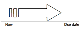
Forward Scheduling:

• Classified based on the time.
• All the activities are scheduled from the date of the planned order release.
• First task of the job is scheduled.
• Its subsequent _task is scheduled on the scheduled completion of the first task.
• Like this, accordingly all the tasks of the job are scheduled.

Backward Scheduling:

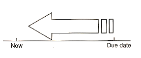
• Also classified based on the time.
• Activities are scheduled from the date or the planned receipt date.
• The last activity is scheduled first.
• Time of the start of the last task is considered as the time for the start of the previous activity.

Forward & Backward Scheduling:

In job shops, where clients place orders on a "need as soon as feasible" basis, forward scheduling (set forward) is widely employed. The start time is determined by forward planning by allocating the earliest available time slot to the next priority job, and from that period defines when the job in that work centre will be completed. Because of the job 'and' Its components begin as soon as feasible, and they are usually completed before the deadline due at the routing's future work centres. The method of set forward generates in process inventory that will be required at successive work centres, as well as increased inventory costs.

When compared to backward scheduling, forward scheduling is simple to use and gets jobs done faster.

Backward Scheduling: (Set backward) is commonly used in assembly industries to commit to specified delivery dates ahead of time. Backward scheduling sets the start and finish times for waiting jobs by allocating them to the most recent available time slot, ensuring that each job is performed exactly when it is due, but not sooner. Backward scheduling reduces inventory by allocating jobs as late as possible. A job is not completed until it must proceed directly to the next work centre on its route.

Single Machine Scheduling:

Illustration: The processing times of jobs on an VMC is given.

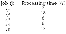
The jobs arranged as per the SPT sequence along with completion times are given in the table. (time in minutes)

Since the preparation or ready time is zero for all the jobs the flow time for all .

Therefore, the minimum flow time minutes.

• Weighted Shortest Processing Time (WSPT)

The importance of jobs in single machine scheduling may vary. In such a situation each job is assigned a weight . The mean flow time computed incorporating the weights is referred to a weighted mean flow time and the computation is,

Processing the jobs in increasing order of weighted processing time is referred to as WSPT.

Illustration:

Jobs are to be arranged in the increasing order of i.e. the lowest first. The optimal sequence that will minimise weighted mean flow time is . The optimal sequence and mean flow flowtime is given in the table:

• Earliest Due Date (EDD)

Lateness of a job is defined as the difference between the completion time and due date of the job.

can be either positive or negative values. The maximum job lateness which is called job tardiness is minimised by earliest due date (EDD sequencing). The sequencing of jobs in single machine scheduling in the increasing order of due dates is known as earliest due date (EDD) rule.

Illustration: Given the following information, processing time and due dates for jobs is given.

Determine the sequence which will minimize the maximum lateness . Determine the corresponding w.r.t. Optimal sequence.

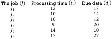
The EDD sequence of the given job is

This sequence gives the minimum value of '

The table below shows the computation of lateness values of jobs as per EDD sequence.
The maximum lateness is 45. This is the minimum value of for optimal sequence.

Dispatching:

Dispatching is the process of starting productive activities by issuing orders and instructions in line with route sheets' previously determined times and sequences.

Functions of Dispatching:

• Dispatching's primary duty is to prepare manufacturing orders, which include shop orders, move orders, tool orders, and so on. These must be distributed to the appropriate individuals at the appropriate times.
• The relevant order and manufacturing forms are released so that operations can begin.
• Take the appropriate quantity of material from the stores and send it to the work centre, where the first operation will be executed via a store issue order.
• The issue of production-related tools.
• Transport between departments (move order).
• Perform a stage inspection.
• Scheduling and coordination.
• Delivering supplies to dispatch or final components warehouses.

Documents Raised by the Dispatcher:

• Requisitions for materials.
• Job cards: These cards authorise a worker to begin work on a certain material, specify what to perform, and serve as a means of tracking production progress.
• Labor cards: These are used to indicate the amount of labour time used and the quantity of work completed, as well as to provide additional information that is needed to prepare production reports and payrolls.
• Move cards: These cards authorise the movement of materials in accordance with the job's requirements and are used in production progress reports.

Duties of a Dispatcher:

• All shop orders and related papers are received and filed.
• Prioritization of jobs for issue in the most advantageous order.
• The distribution of job cards or other types of operational instructions.
• 4, Provide setters with instructions on which machines to start up, for which jobs, and when.
• Distribution of instructions for moving items between work centres.
• Issue of instructions for the issue and return of special tooling to retailers.
• Keeping track of production records.

2.10 Concept of JIT manufacturing system

Just-in-time (JIT) inventory management is a strategy for aligning raw-material orders from suppliers with production schedules. Companies use this inventory technique to improve efficiency and avoid waste by acquiring products only as needed for the manufacturing process, lowering inventory expenses. This strategy necessitates producers precisely forecasting demand.

Working:

The just-in-time (JIT) inventory system reduces inventory and boosts productivity. JIT manufacturing systems reduce inventory costs by allowing manufacturers to obtain supplies and parts only when they are needed, eliminating the need for storage. If an order is cancelled or not completed, manufacturers are not left with unsold inventory.

A vehicle manufacturing that runs with minimal inventory levels but significantly relies on its supply chain to deliver the parts it needs to produce automobiles on an as-needed basis is an example of a JIT inventory system. As a result, the manufacturer only orders the parts needed to assemble the automobiles after receiving an order.

Advantages & Disadvantages:

Compared to traditional inventory models, JIT inventory systems have a number of advantages. Short production runs allow firms to easily switch from one product to the next. This strategy also saves money by reducing the requirement for warehouse space. Companies also spend less money on raw materials because they just buy what they need to manufacture the things they've ordered.

The downsides of JIT inventory systems include the possibility of supply chain disruptions. If a raw-materials supplier goes down and is unable to deliver the goods on time, the entire manufacturing line could be halted. The delivery of finished items to end clients may be delayed if an unexpected order for goods is placed.

What is JIN:

A just-in-time (JIT) inventory system is a business approach that involves receiving products as close to when they are needed as possible. As a result, if a car assembly facility wants to install airbags, it does not have a supply of airbags on hand, but instead orders them as the cars come off the assembly line.

A key benefit of a JIT system is that it reduces the need for a company to keep large amounts of inventory on hand, resulting in increased efficiency and significant cost savings. A supply or demand shock, on the other hand, can bring everything to a halt.

2.11 Project Management: Project network analysis

The approach of network scheduling is used to plan and schedule major projects in the domains of construction, maintenance, fabrication, and other sectors. This methodology involves identifying essential components and organising numerous processes to reduce bottlenecks, delays, and interruptions. There are two primary methods for planning and controlling your project. Critical Path Method (CPM) and Program Evaluation and Review Techniques are two of them (PERT).

Objective:

• A powerful coordinating tool for planning, scheduling and controlling of projects.
• Minimisation of total project cost and time.
• Effective utilisation of resources and minimisation of effective resources.
• Minimisation of delays and interruption during implementation of the project.

Application:

• Research and development projects
• Equipment maintenance and overhauling
• Construction projects (building, bridges, dams)
• Setting up new industries
• Planning and launching of new products
• Design of plants, machines and systems
• Shifting the manufacturing location from one location to another
• Control of production in large job shops
• Market penetration programmes
• Organisation of big programmes, conferences, etc.

Basic concepts:

• Network: A network is a graphical depiction of a project that consists of a series of activities organised in a logical sequence and depicting the interrelationships between them.
• An activity is a physically identifiable aspect of the project that takes time and resources to complete. Each action has a distinct beginning and end point. An arrow is used to signify activity ()
• The beginning or end of an activity is represented by an event. An activity's start and finish points are called events.

Example: Machining a component is an activity

Start Machining is an event

Machining completed is an event

Several activities in a network may merge into a single node, known as a merge node, and a number of activities may emerge from a single node, known as a burst node.

The merge and burst events are depicted in

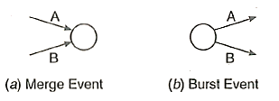
• Predecessor and Successor Activities: Predecessor activities are all those activities that must be done before beginning the activity in question.

All actions that must occur after the activity in question are referred to as successor activities.

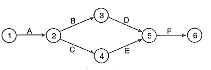
Activities 2-3 and 2-4 are immediate successors to activity 1-2.

Activities 2-3 and 2-4. 3-5, 4-5 and 5-6 are its successor activities.

Activities 1-2, 2-3, are predecessors to activity 3-5 and 2-3 is the immediate predecessor.

The precedence relationship between the activities can be expressed as,

• Path: A path is an uninterrupted line of activities that connects two events. As an example, look at the diagram above. The path A-B-D-F connects occurrences (1) and (6). The network has several paths identified across it.
• Dummy Activity: An activity that simulates a dependency or relationship but does not take up time or resources. It's used to keep track of the logical order. A dotted line is used to signify it. A dummy activity is depicted in

Consider the network of activities P, Q, R and S, activity R is preceded by activities P and Q. While activity S is preceded by Q only. The wrong and correct representation of

These activities are shown,

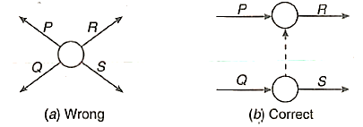
Numbering of events:

The stages for counting events according to Fulkerson's rule are as follows:

1. The first event is numbered "1" since it has all outgoing arrows but no incoming arrows.

2. Remove all arrows emanating from node "1." This will turn a few additional nodes (at least one) into initial events, which will be numbered 2, 3,, and so on.

3. To make more initial events, delete all the arrows that go out from these numbered events. Assign these events new numbers.

4. Continue until the final or terminal node is numbered, with all arrows coming in but none going out.

2.12 CPM

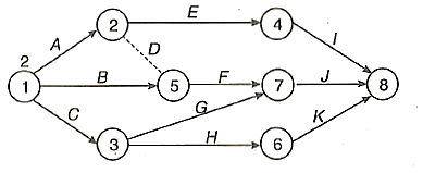
The activity times are known with certainty in the Critical Path Method (CPM). The earliest start time (EST) and latest start time (LST) for each activity are calculated. "The crucial path is the one with the longest time sequence. The critical route length specifies the shortest period in which the project may be finished. 'Crucial activities' are the activities on the critical route." " The goal of the time analysis in the network is to:

1. Calculating the project's completion date

2. The earliest possible start time for each activity

3. The latest time when each activity can begin without causing the entire project to be delayed.

4. Choosing the appropriate float for each activity

5. The critical activities and critical path must be identified.

Forward Pass Computations (Earliest Event Time):

1. Calculating the project's completion date

2. The earliest possible start time for each activity

3. The latest time when each activity can begin without causing the entire project to be delayed.

4. Choosing the appropriate float for each activity

5. The critical activities and critical path must be identified.

Earliest Start time (ES):

It is the earliest event time of the tail end event

Were,

Earliest Finish time (EF):

Starting time + Activity time

Earliest event time:

For event 'j’ is the maximum of the earliest finish times of all

Activities ending into that event

Backward Pass Computations (Earliest Event Time):

The latest event times define the deadline by which all activities in that event must be completed without causing the project to be delayed.

• Latest finish time for an activity )equals the latest time of event

• Latest starting time of activity is the latest completion time of minus the activity time.

• Latest event time for event i is the minimum of the latest start time of all activities originating from that event.

• Slack - The slack of an event is the difference between the latest and earliest event times

The events with zero slack time are known as critical events.

• Floats

• Total Float: It is concerned with the entire duration of the project. "The length of time that an activity can be delayed beyond its earliest projected completion time without affecting the overall project duration time," according to the definition.  The difference between the latest and earliest start times for an activity is the total float for that activity.

• Free float

It's the amount of time that an activity's completion can be postponed beyond its earliest end time without influencing the earliest start of a subsequent activity.

• Independent float

It is the length of time that an activity's start can be postponed without influencing the earliest start time of any subsequent activities, providing that the preceding activity has completed at its latest end time.

Example 1:

Construct the network diagram

Solution:

The critical path is one that connects the activities with zero slack. The critical paths

A-B-D-F-G

Example 2:

Find the floats for each activity

Solution:

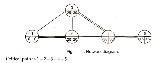
Activity	Duration	Earliest		Latest		Float
		Start	Finish	Start	Finish	Total	Free	Independent
	20	0	20	0	20	0	0	0
	25	0	25	5	30	5	5	5
	10	20	30	20	30	0	0	0
	12	20	32	24	36	4	4	4
	6	30	36	30	36	0	0	0
	10	36	46	36	46	0	0	0

Example 3:

Activity	Immediate Predecessor	Activity Time (Weeks)
		12
		20
		28
		12
		28
		12
		8
		8

Solution:

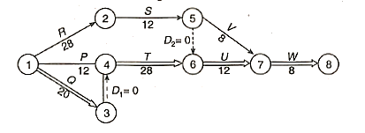
Activity	Duration	ES	EF	LS	LF	Slack
P	12	0	12	8	20	8
Q	20	0	20	0	20	0
R	28	0	28	8	36	8
S	12	28	40	36	48	8
T	28	20	48	20	48	0
U	12	48	60	48	60	0
V	8	40	48	52	60	12
W	8	60	68	60	68	0
	0	20	20	20	20	0
	0	40	40	48	48	8

The critical path is: Q -T – U – W

Project duration = 20 +0 + 28 + 12 + 8 =68 weeks

2.13 PERT and Project crashing

There is only one time estimate in the Critical Path Method. As a result, it ignores time uncertainty. In fact, activity duration may not be deterministic (certain) in every case. The uncertainty of activity times is considered by PERT. It's a probabilistic model with activity duration uncertainty.

PERT makes use of three estimates of time:

1. Optimistic time

2. Most likely time

3. Pessimistic time

• Optimistic time is the shortest time that can be achieved if everything goes according to plan and there are no difficulties. It's an estimate of the shortest time it would take to accomplish the activity in perfect conditions.

• The most likely time is the most accurate time estimate for the action. This time estimate is in the middle between the optimistic and pessimistic ranges.

• The pessimistic time is the longest time when all odds are considered. If everything goes wrong, this is how long it will take.

The three-time estimates are combined to develop expected time for an activity. The fundamental assumption in PERT is that the three estimates of time follow (Beta) distribution.

Standard deviation of the time required to complete each activity,

Standard deviation of the time to complete the project,

Probability of Completion of the Project within a Scheduled Time:

The likelihood of finishing a project is determined by the probability of the network's end event occurring. The normal distribution is assumed for the probability distribution.

The probability of completion of the project within scheduled is computed as:

1. Calculate the mean of the event time by adding the times of the activities along the critical path leading to the event.

2. Calculate the variance of the event time by adding up the variances of the activities on the critical path. Take the squire root of this variance to get T (standard deviation).

3. Compute standard normal variate,

From tables of normal curve, the value corresponding to Z gives the required probability.

Example 4:

Construct the PERT Network—Find the critical path and variance of each event. Find the project duration at 95 per cent probability

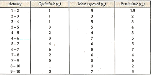
Solution:

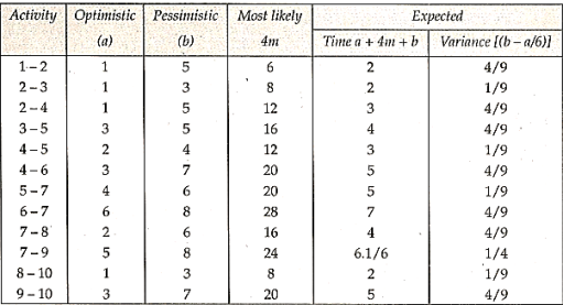
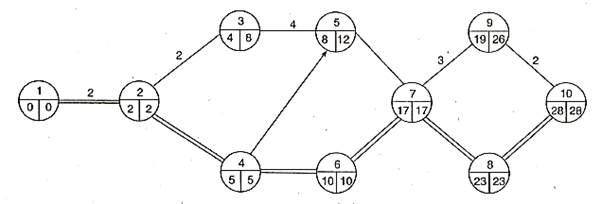
Project management is a structured approach to planning, scheduling, executing, monitoring, and controlling the many phases of a project. PERT and CPM are two project management approaches that every project management should use to meet their project deadlines. These methods allow you to see how your project is progressing as well as a sequence of actions and events.

Project Crashing:

Direct and indirect expenditures will make up the total overall cost. Overheads, office expenses, administrative charges, cost penalty for late work, and so on make up the indirect cost, the indirect time changes with time. Any time saved on a project implies less money spent on indirect costs.

The cost of supplies, machinery employed in the project, and payments for labour and subcontracting are all considered direct costs.

It is assumed that there is an activity duration for which the direct cost is lowest for each activity. If the activity takes longer than this, more resources and, as a result, more finances are necessary. For example, regardless of resources used, a point will be reached beyond which no further reduction in time will be feasible. Normal time is the time required to do an activity at the lowest cost, while crash time is the time required to complete the action at the lowest cost. Normal and crash costs are the costs associated with these times. Time and cost are expected to have a linear relationship, as indicated.

Procedure for crashing

Crashing is a technique for shortening the duration of a project. The crashing occurs at the expense of additional resources, i.e., at a cost.

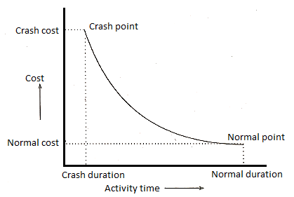
The steps to prevent a project from crashing are as follows:

1. Create a network diagram and identify the critical path for each network diagram.

2. Determine the cost slope for various activities.

3. Crashing the network — crashing important path activities according to their ranking, i.e., the activity with the lowest cost slope would be crashed first and to the greatest extent possible.

4. Calculate the project's overall cost.

Example 5:

Indirected cost = 70 per day

Solution: The network is shown in the Fig. Along with earliest and latest starts.
 

Direct cost of the project & 580

Indirect cost of the project र 1260

Total project cost 1840

The cost slope

Fig. Network diagram with ES and LS.

The cost-slope is shown.

Instead of crashing all the activities, only those activities whose cost slope is less than the indirect cost.

Along the critical path activities , both activities and have cost-slopes less than indirect cost.

The minimum cost slope is associated with , and it can be crashed by two days.
Project duration is reduced to 16 days while critical path remains unchanged

Direct cost

Indirect cost

Total cost

Network after crashing is shown in Fig

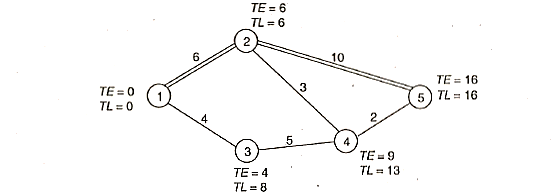
Next, crash the activity 2-5 by 5 days

The critical path is changed to 1-3-4-5. This is the shown in the fig. 27.14

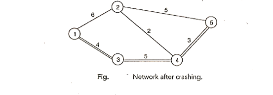
Activity on new critical path (Slope less than 70 are and ) crash on new critical the activity by days.

Critical path again chances to

Total cost

This is shown in Fig.

Fig. Network after crashing.

The project cannot be crashed any further as the activities on the critical path are already crashed. From the network diagram, the activity can be expended by one day without affecting the project duration.

This will save crashing cost of activity for one day

Total cost

Optimal project duration days

Optimal project cost

Comparison between CPM and PERT:

Key Takeaway:

References:

1. Industrial Engineering and Production Management by Martand T Telsang S. Chand Publishing
2. Operations Research Theory & Applications by J K Sharma, Macmillan India Ltd,
3. Automation, Production Systems & Computer Integrated Manufacturing by Groover, M.P. PHI
4. Operations Research by P. K. Gupta and D. S. Hira, S. Chand & Co.