Unit - 5
Operational Analysis
When there are several uses of resources, linear programming is a mathematical technique for determining the best allocation of resources and achieving a specific goal. Cost minimization or profit maximisation may be the goal.
In practise, one of the most effective techniques for managerial decision-making is linear programming. The adoption of this technique has aided in the resolution of numerous complex situations that would have been more difficult to resolve otherwise. The following are some examples of problems where this strategy can be used successfully:
• Production scheduling
• Product mix decisions
• Capital budgeting
• Plant location
• Resource allocation and optimal utilisation of resources
Product mix decisions:
The choice of product mix is a crucial planning task. The best product mix selection has far-reaching ramifications and contributes to an industry's survival and success.
There are numerous constraints that must be considered while deciding on product mix, including cost, capacity, and other factors.
The linear programming problem (LPP) is a method for determining the best product mix.
Linear programming is a quantitative technique in which the relationships between variables in a problem are linear, thus the name.
Standard form of linear programming problem:
Let  are the decision variables Optimise (maximise or minimise)

Subject to constraints.


The LPP can be Solved by Two Method:
• Graphical technique: This method is only utilised when there are two choice variables. This is a lot easier.
• Simplex method: This is beneficial when there are a lot of choice variables in the problem and a lot of restrictions.
Formulation of LP problem:
In the formulation process, there are several steps.
• Determine the most important decision to be made based on the problem.
• Determine the choice variable...... Whose values determine the problem's solution.
• Express the goal as a function of linear variables and write it in quantitative terms.
• Analyse the constraints and write them down as a set of linear equations.
Example:1:
A form can make three varieties of cloth, A, B, and C, and it requires three types of wool, red wool, green wool, and blue wool. 2 yards of red wool and 3 yards of red wool are required for one unit length of type A cloth. 3 yards of red wool, 2 yards of green wool, and 2 yards of blue wool are required for one unit length of type B cloth, while 5 yards of green and 4 yards of blue wool are required for one unit length of type C cloth. Only 8 yards of red, 10 yards of green, and 15 yards of blue wool are available on the form. The profit from the sale of one unit length of type A is ten rupees, eight rupees for type B, and five rupees for type C.
Determine how the firm should use the available material to. Maximise the profit. Formulate this as a LP problem.
Solutions:
• They key decision here to find the units of three type of cloths A, B and C type to be produced by the company.
• Let  be the number of cloths of type A, type B and type C to be produced respectively.
• The objective is to maximise the profit by selling three types of cloths.
• The profit equation is written as

Here the coefficient represents the contributions towards the profit equations.
• Requirements and availability of wool.

These can be expressed as a linear equation.


These are represented in standard from as:

Subjected to,


Example:2:
Rolls of paper for cash registers are manufactured by a paper manufacturer. Each roll of paper is 200 metres long and comes in widths of 2.5, 5, 7.5, and 12.5 centimetres. The company's manufacturing technique yields 200 metres of 30 cm wide rollers. The corporation needs to cut their 30-centimeter roll to the necessary width. It comes with six basic cutting options.
Cutting Alternative |
| Number of Rolls | Waste (cms) | ||
| 2.5 | 5 | 7.5 | 12.5 |
|
1 | 6 | 3 | 0 | 0 | 0 |
2 | 0 | 3 | 2 | 0 | 1 |
3 | 1 | 1 | 1 | 1 | 1 |
4 | 0 | 0 | 2 | 1 | 1 |
5 | 0 | 4 | 1 | 0 | 1 |
6 | 4 | 2 | 1 | 0 | 1 |
The maximum demand requirements for the 4 rolls are as follows:

The company wishes to minimise the waste created by its production process, while meeting its requirements.
Formulate the problem as a LP model.
Solution:
Let  be the number of cutting alternatives
Where,

 is the waste produced in alternatives 3, 4, 5 and 6 respectively.
Minimize,

Subjected to,


Step I: Express the problem mathematically.
Step II: Draw the problem constraints on a graph, temporarily ignoring the inequality sign, and determine the region of feasibility based on the inequality sign of the constraints. The shaded area, which forms a convex polyhedron, indicates the area of the possible solution.
Step III: Calculate the coordinates of all points in the feasible solution's corner.
Step IV: Determine the value of the goal function that corresponds to all of the solution locations identified in step three (III).
Step V: Find a plausible solution that maximises the objective function's value.
Example:3:
A firm makes two different sorts of dolls: A and B. Dolls A and B are of higher quality, whereas Dolls C and D are of poorer grade. Profit on doll A is Rupee 5 whereas profit on doll B is Rupee 3. Each doll A requires twice the amount of raw material as doll B. The raw material supply for doll B is limited to 1000 per day. Doll A need a unique crown, and only 400 of these clips are accessible each day. Only 700 crowns are available per day for doll B. Find the product graphically such that the corporation makes the most profit.
Solution:
The formulation of the LPP. Is

Subjected to,


The straight lines corresponding to the constraint equation are plotted
Equation 1:


Equation 2:

The co-ordinates are (0.400,0)
Equation 3:

The co-ordinates are (0, 700)
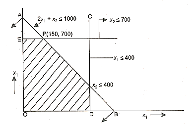
The co-ordinates of the corner point are,

Then substituting the values off these points in objective function the maximum value is got for point P (150, 700)
The value of Z = 2050.
150 number of doll A and 700 number of doll B are to be produced to maximise the profit.
Example:4:
Find the optimal solution to the LP problem given using graphical method

Subjected to:


Solution:
This is a minimisation problem. The constraint equation is (making them equalities).
Equation 1:


Co-ordinates are (0, 24), (8, 0)
Equation 2:

Co-ordinates are (0, 16) (16, 0)
Equation 3:


Co-ordinates are (0, 8), (24, 0)
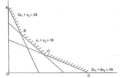
The values of objective function
Point | Co-ordinate | Objective function Value (z = 600   |
A | (0,24) | 9600 |
B | (4,12) | 7200 Minimum |
C | (12,4) | 8800 |
D | (24,0) | 14600 |
The optimal value of objective function 14,600
The optimal solution is 
• In standard form, formulate the problem as an LPP problem.
• As required by the situation, convert the inequalities into equalities by introducing slack or surplus and/or artificial variables.
• Get the initial or starting solution by setting n-in variables in the problem, where m denotes the number of constraint equations. Non-basic variables are called basic solutions, while variables set to zero are considered non-basic variables. Those (n-m) variables should be set to zero, resulting in a one-of-a-kind solution to the problem.
• The initial solution is tabulated and is referred to as the initial simplex Table.
• The solution is then improved by the number of iterations until the best solution is found.
This step is explained as follows:
Determine the entering variable: The entering variable is the variable with the most negative value in the z equation of the initial Table. As it enters the basis, this is referred to as entering variable.
Leaving variable: This is the variable that leaves the basis for a new entering variable to take its place. To find the leaving variable, calculate the ratio of entering column co-efficient for all rows except the z (objective) row, which only considers +ve values. The leaving variable is the one associated with the least ratio.
The column that corresponds to the variable being entered: It's referred to as the "entry column" or "pivot column." The pivot row is the row that corresponds to the leaving variable. The pivot element or key element is the element at the junction of the pivot row and pivot column.
When calculating the improvement, the pivot element should be 1 and the pivot column should contain zeros in all other places. The Gauss-Jordan elimination method is used for this.
The new values are calculated using the following equations.

New Z equation = (Old Z equation) - (its entering column coefficient) x new pivot equation.
For all other equations, (old equation) - its entering column co-eff x New Pivot equation.
The values obtained as represented in the Table.
• Test for optimality: If the values of the non-basic variable in Z row are all +ve, then optimal solution is reached.
Get the value of Z and decision variables from the Table otherwise Repeat step 5 to get the improved solution till optimal solution is obtained
Example:5:
Painting, assembly, and testing are the only three processes performed by a company that manufactures two items A and B. The necessary product information is listed below.
Product | Sales price (per unit) | Hours required per unit | ||
Assembly | Painting | Testing | ||
A | 50 | 1.0 | 0.2 | - |
B | 80 | 1.5 | 0.2 | 0.1 |
Total number of hours available each week are:
Assembly — 600 Hrs., Painting — 100 Hrs., Testing — 30 Hours.
The firm wishes to determine its weekly production to maximize its revenue.
Formulate the model and solve by simplex method.
Solution:
Let,  be the number of units of product A and B respectively to be produced in order to maximise revenue
The problem can be represented as an LPP, model as shown below:

Subjected to:


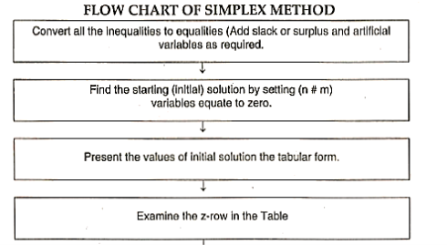
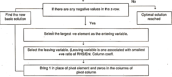
Simplex procedure:
- Initial or Starting Solution: The problem can be rewritten by introducing slack variables to convert inequalities into equalities.
The problem after introducing slack variable can be written as,

Subjected to:


Number of variables (n) = 5
Number of equations (m) = 3
To get the starting solution, (n-m) variables should be set equal to zero. The variables
Set equal to zero should be such that they should give a unique solution.
(n-m) = 5 - 3 = 2 variables
Two variables,  should be set equal to zero.
Substituting which gives:


The starting solution is represented in the form of an initial Table
Pivot Column | |||||||||
| Basic | Z |  |  |  |  |  | Solution | Ratio |
| Z | 1 | -50 | -80 | 0 | 0 | 0 | 0 | - |
|  | 0 | 1 | 1.5 | 1 | 0 | 0 | 600 | 400 |
|  | 0 | 0.2 | 0.2 | 0 | 1 | 0 | 100 | 500 |
Pivot row |  | 0 | 0 | 0.1 | 0 | 0 | 1 | 30 | 300 |
The variables which are set equal to zero  are called non basic variables and variables which are not set equal to zero are called basic variables
Ilteration:1:
The highest negative value in the z - row is associated with the variable x2. So x2 is the entering variable.
To find out the leaving variable, the ratio of

Only for +ve coefficients of the entering column the ratio is to be calculated. The ratio is to be calculated only for constraint equation.
The minimum positive ratio is 300 associated with variable x5 so x5 is the leaving variable.
The pivot element should be 1 and the other coefficient in pivot column should be zero.
The get this, Gauss-Jordan elimination method is used, or the following equations are used to calculated new equation

New z-equation = old z equation - (its entering column coefficient) x NPE
Other equations can be calculated as,
New equation = old equation - (its entering column coefficient) x NPE
Basic | Z |  |  |  |  |  | RHS | Ratio |
Z | 1 | -50 | 0 | 0 | 0 | 800 | 2400 | - |
 | 0 | 1 | 0 | 1 | 0 | -15 | 150 | 150 |
 | 0 | 2.0 | 0 | 0 | 1 | -2 | 40 | 200 |
 | 0 | 0 | 1 | 0 | 0 | 10 | 300 | - |
Ilteration:2:
The Variable x1 (which has the coefficient of -50 in z-row) is the entering element. To determine the leaving variable, the ratio of

The ration corresponding to the variable x3 is minimum (150) x3 is the leaving variable.
Now, if there is already 1 in the position of pivot element there is no need to compute the new pivot equation.
The z-equation and x4 and x2 equations are calculated and the value are tabulated as
Basic | Z |  |  |  |  |  | Solution |
Z | 1 | 0 | 0 | 50 | 0 | 50 | 31,500 |
 | 0 | 1 | 0 | 1 | 0 | -15 | 150 |
 | 0 | 0 | 0 | -0.2 | 1 | 1 | 10 |
 | 0 | 0 | 1 | 0 | 0 | 10 | 300 |
Since all the non-basic variables in the z-equation (row) are non-negative, optimality has reached.
The solution is,


Substituting these values in objective function.

Big M Method:

 ,
,


Solve the problem using simplex method.
Step 1:


Step 2:
Set the (n-m) variable equal to zero to get the starting.
No of variables = 6
No of constraint equations = 3
(n-m) = 6-3 = 3 variables should be set equal to zero i.e., x1, x2 and x3 should be equal to zero to give in the unique solutions.
Substituting these values in constraint equations we get the initial solution.
A = 2
x4 = 3
X5 = 5 and Z = 0
Objective function is written as,

Pivot row  | Basic |  |  |  |  |  |  |  | RHS | Ratio RHS |
Ent column coefficient | ||||||||||
 | 1 |  | 1 | 0 | 0 | 0 |  | 0 |
| |
 | 0 | 2 | 1 |  | 0 | 0 | 1 | 2 | 1 | |
Pivot element |  | 0 |  | 3 | 0 | 1 | 0 | 0 | 3 | 3 |
|  | 0 | 0 | 1 | 0 | 0 | 1 | 0 | 4 |  |
x1 is the entering variable (as it has max -ve value in z-equation)
Entering column coeffs.
To find out the leaving variable, the ratio of

The minimum positive ratio (1) corresponding to Al is the leaving variable.
The pivot element is 2 (Element at Intersection of pivot row and pivot column)
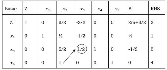
For the next step, x3 is selected as a entering variable (most -ve value in z-equation). And x4 is the leaving variable as it is the only variable associated with minimum positive ratio (2/y2) = 4
The point element is to be made 1 and all other elements in the column are to be made as zero using the Gauss Jordan elimination method or by using the equations
To improve the solution, there should be 1 in the place of pivot element and zeros in the other places in the column.
This is obtained by Gauss-Jordan elimination method or by calculating the equations using formulas
1. New pivot equation = 

2. New z-equation=Old z equation – its entering coeff. × NPE
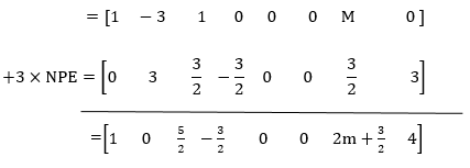
3. Other equations are calculated as
New equation =Old equation – (its entering column coeff. ×NPE)
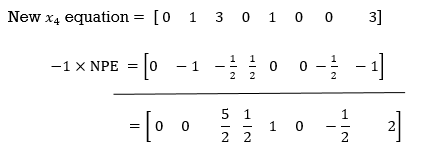
x5 equation has already zero in the pivot column So, it remains unchanged.
These values of new equations are represented
Basic | Z |  |  |  |  |  | A | RHS |
Z | 1 | 0 | 10 | 0 | 3 | 0 | M | 9/2 |
 | 0 | 1 | 3 | 0 | 1 | 0 | -1/2 | 3/2 |
 | 0 | 0 | 5 | 1 | 2 | 0 | -2 | 1 |
 | 0 | 0 | 1 | 0 | 0 | 1 | 0 | 4 |
Since the value of coefficient of non-basic variables are +ve the optimality has reached the optimal solution is,

Value of decision variables.

Substituting these values in objective function,


Maximum value of objective function =9/2
Duality in LPP:
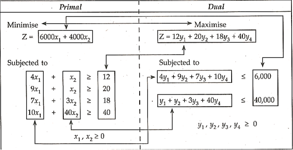
Every linear programming issue, whether it is one of maximisation or minimization, has a mirror image problem based on the same data. The primary problem is known as the primal problem, whereas the secondary problem is known as the dual problem.
Formulation of dual from the primal problem.
- If the primary problem is a maximisation problem, the secondary problem will be a minimization problem, and vice versa.
- The total number of primal decision variables equals the total number of dual constraints, and the total number of dual variables equals the total number of primal constraints.
- In the primal problem, the profit constraints Cj replace the capacity constraints bi, and vice versa, i.e., the coefficients in the primals objective function are replaced by dual constraints, and vice versa.
- If the inequalities in the primary problem are of type
 , they are of type
  in the dual problem, and vice versa.
 - Ignoring the non-negativity constraints, if the primal problem has 'n' variables and m inequalities, the dual problem will have m variables and n constraint equations (inequalities).
- The signs in the non-negativity constraints are
 both in primal and dual problems.
 - The coefficients are positioned column wise [from top to bottom] in the dual’s constraint inequalities row wise (from left to right) and vice versa in the dual’s constraint inequalities.
- The dual problem's coefficient matrix of constraints is the primal's transpose.
Characteristics of Duality:
- A basic problem is the dual of the dual.
- If one of the primal or dual problems has a solution, the other must as well, and their optimal values must be the same.
- The objective function value for any viable primal solution is less than the objective function value for any feasible dual solution.
- If either the primal or dual problem has an infinite solution, the problem is impossible to solve.
Advantages of Duality:
- The dual solution verifies the accuracy of the primal solution by looking for computational mistakes.
- Problems with more constraints than variables necessitate greater computational work than problems in which the number of variables outnumbers the number of constraints. Because the number of iterations in the simplex technique is proportional to the number of rows, this is the case. As a result, solving the problem's dual, which has more constraints than variables, would be preferable.
- Provides information on how the optimal solution varies when the coefficients and problem formulation vary (sensitivity analysis).
- The dual's economic interpretation aids management in making future decisions.
A linear programming issue can be addressed under certain limitations, and cost coefficients may not be the same or stable for an extended period of time. Markets fluctuate, material costs, and labour costs change over time, and the best solution obtained based on a single estimate rarely reflects reality. This form of uncertainty is frequent in the corporate world, and it is necessary. To determine the impact of such changes on the model's input parameters It is critical to verify the solution's validity range.
"Post-optimality analysis or sensitivity analysis" is the term for the inquiry of this. It is not required to search for the outcome once it has occurred in reality. When it comes to changing the prices of items, the decision maker can make a better decision if he knows that a Rupee 1 increase in the selling price of one product results in a bigger profit than a similar increase in the selling price of the other product.
The analysis is not halted after discovering the optimal solution to the LP problem; it is extended to sensitivity analysis or post-optimal analysis to gain a good understanding of the problem.
Basic Principles of Sensitivity:
- In the final tableau of the original problem, explain the modifications caused by the new problem.
- Check to see if the identity matrix is still there in the tableau after the changes have been made. If it doesn't, row operations should be used to obtain the identity matrix.
- Determine whether the solution is viable. This is determined by looking at whether the variable values are positive or negative. Bring the solution into viability if they aren't already.
- Check to determine if the solution is optimal if it is practicable.
The approach to sensitivity analysis in terms of the effect on the optimal solution with the following changes.
Change in the coefficient of the objective function: Consider that the objective function has changed from

Subjected to same constraints


Now, the coefficient of x1 has changed from 3 to 4.
The incremental change in the co-efficient in the objective function is (4 - 3) =1 while doing iterations in simplex method, we bring the variables from RHS to LHS in the Z-equation. So, the incremental change in the coefficient of x1 in LHS is -1. This change i.e., introduction of Coeff. Of x1 = -1 in 1-eqn, will not give the identity matrix. To get the identity matrix row operation is carried out and the optimal solution is worked out.
- Changes in the RHS of the constraint: This helps to indicate the extent of increase of RHS quantities without altering the existing basic variables. e.g., consider the constraint in (a)
 has changed to
  . Now changes will take place only at
RHS.
b. Changes in the coefficient of the constraints: e.g., the problem in (a), if the coefficient of x1 has changed due to new labour force added i.e., has changed to
c. Determine the series of fundamental conditions that become optimal as the LP parameters are changed more and farther. The goal of this analysis is to figure out 'how sensitive the optimal solution is to changes in the parameters.' Sensitivity analysis is the term for this type of investigation.
Degeneracy
When one or more basic variables in linear programming have zero values, it is said to be degenerate. Degeneracy can occur
- At the beginning of the process when at least one basic variable in the initial basic viable solution is zero. If the right-hand side of a constraint is zero, this will be the case.
- At any later iteration step when the minimal non-negative replacement ratios are tied. It is frequently proposed that the outgoing variable be chosen at random. The other tied variable will become 0 in the next table, indicating that the solution is degenerate.
There is no guarantee that the goal function's value will improve, as the new solution could still be degenerate. The simplex method's efficiency is severely harmed as a result of this. Cycling, or 'circling,' is a more dangerous problem in which the same sequence of simplex iterations is repeated indefinitely without improving the solution. Fortunately, cycling-related issues are extremely uncommon. In fact, it's difficult to think of a situation when cycling occurs.
However, by using the following basic process, dubbed the perturbation method by A. Charnes, the number of iterations required to obtain an optimal solution can be lowered.:
- Multiply the positive coefficients of the key-column in each tied row by each element.
- From left to right, compare the resulting ratios, column by column, in the identity and then in the body of the simplex table.
- The outgoing variable is found in the row with the smallest algebraic ratio. The simplex approach is then used to find the best solution.
The approach outlined above can be used to any iteration. If any artificial variable is one of the tied variables, it should be picked to leave the basis immediately rather than pursuing the aforesaid approach.
So, with the exception of a minor inconvenience, dealing with a degenerate solution is not frightening. The criterion demonstrates that the problem has at least one redundant restriction from a practical standpoint. As a result, the appropriate resources are unnecessary. The understanding that some resources are unnecessary can be useful throughout the solution's implementation.
A few examples will now be used to explain the phenomena of degeneracy resolution.
Note for Simplex:
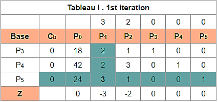
The first row consists of the objective function coefficients, while the last row contains the objective function value and reduced costs Zj - Cj.
The last row is calculated as follows: Zj = Σ(Cbi·Pj) for i = 1..m, where if j = 0, P0 = bi and C0 = 0, else Pj = aij. Although this is the first tableau of the Simplex method and all Cb are null, so the calculation can simplify, and by this time Zj = -Cj. See the example below
Maximize 
Subject to 


Example 6:


Solution:
Step 1: Set up the problem in the standard Form


Note that there is no need to introduce artificial variables as x1 and x2 are themselves forming identity matrix  and can be treated as basic variables.
Step 2. Find an Initial Basic Feasible Solution
Setting x3 = 0, the basic feasible (degenerate) solution to the problem is


|  | 2 | 3 | 10 |
|
|
 | Basis |  |  |  |  |  |
2 |  |  | 0 | (2) | 0 | 0  |
3 |  |  | 1 | 1 | 1 | 1 |
|  |  | 3 | 7 | 3 |
|
|  |  | 0 | 3  |
| Initial b.f.s |
Step 3: Perform Optimality Test
Since  is positive under x3 column
Step 4: Iterate Towards an Optimal Solution
Performing iteration to get an optimal solution result in the following table
|  | 2 | 3 | 10 |
|
 | Basis |  |  |  |  |
10 |  |  | 0 | 1 | 0 |
3 |  |  | 1 | 0 | 1 |
|  |  | 3 | 10 | 3 |
|  |  | 0 | 0 | Optimal b.f.s |
Is optimal and the optimal b.f.s. is


The above solution is, however, degenerate because basic variable x3 has zero value. Note that the value of Z in Step 2 as well as Step 3 is same. Thus, we have obtained the optimal degenerate solution from a degenerate solution without improving the value of Z. In other words, it is possible to move from one table to another without any improvement in the objective function.
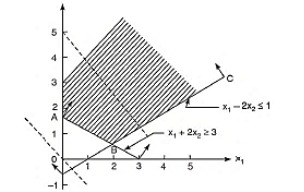
Unbounded solution: When the restrictions on an L.P. Issue have no limit, the viable region is not constrained in any way. In the unbounded feasible zone, variables x1 and/or x2 can have any value, and their value/values can theoretically increase to infinity. The objective function's value can be finite or infinite. The problem is said to have an unbounded solution when it is endless. The solution's unboundedness implies that the problem hasn't been properly articulated. While developing the L.P. Model, one or more limitations were mistakenly overlooked.
Maximize 
Subject to


Infeasible solution: When there is no solution to an L.P. Issue that fulfils all constraints and non-negativity restrictions, it is said to be infeasible. It signifies that the problem's restrictions are incompatible and inconsistent. Infeasibility is purely determined by the restrictions and has no bearing on the objective function.
Key takeaway
1. Graphical technique: This method is only utilised when there are two choice variables. This is a lot easier.
2. Simplex method: This is beneficial when there are a lot of choice variables in the problem and a lot of restrictions.
To find out the leaving variable, the ratio of


Every linear programming issue, whether it is one of maximisation or minimization, has a mirror image problem based on the same data. The primary problem is known as the primal problem, whereas the secondary problem is known as the dual problem.
When one or more basic variables in linear programming have zero values, it is said to be degenerate. Degeneracy can occur
Unbounded solution: When the restrictions on an L.P. Issue have no limit, the viable region is not constrained in any way.
Infeasible solution: When there is no solution to an L.P. Issue that fulfils all constraints and non-negativity restrictions, it is said to be infeasible
Assignment Model:
The goal of assignment issues is to allocate an equal amount of resources (men, machines, etc.) to an equal number of jobs at the lowest possible cost. The assignment will be completed one-on-one.
There are n jobs to process, and there are n machines available to do so. The cost of assigning work I to machine j is represented by Cij. The work assignment should be done in such a way that each job is assigned to only one machine. The issue is determining the appropriate work assignment to machines that results in the lowest total processing cost.
Assumption:
- Only one job should be allocated to each machine.
- Jobs differ in their work contents and machines differ in their capabilities.
- The cost of processing each job on each of the machines (Cii) is known.
Mathematical statement of the problem
Minimize 


Subjected to the following restrictions  if the ith jb is not assigned to jth machine and
  if the ith job is assigned to jth machine.

Only one person should be assigned to jth job.

(Only one job is done by jth person)
Hungarian Method for Solving Assignment Problem:
Example 1:
Different jobs are to be done on 4 different machines. The matrix below gives the cost (in Rupee) of producing each job i on each one of the machines j. How should the jobs be assigned to the machine so that the total cost is minimum.
Jobs | Machines | |||
 |  |  |  | |
 | 5 | 7 | 11 | 6 |
 | 8 | 5 | 9 | 6 |
 | 4 | 7 | 10 | 7 |
 | 10 | 4 | 8 | 3 |
Solution:
1. Row Operation: Select the smallest element from each row and subtract it from all other elements from that row. Resulting matrix is
|  |  |  |  |
 | 0 | 2 | 6 | 1 |
 | 3 | 0 | 4 | 1 |
 | 0 | 3 | 6 | 3 |
 | 7 | 1 | 5 | 0 |
2. Column Operation: Select the smallest element in each column and subtract it from all other elements of the column. The reduced matrix after column operation is

3. Make the assignments and draw the minimum number of lines to connect all zero. As the number of lines required to connect all zero (  is less than number of rows or columns. Then proceed further to step 4
4. Select the smallest element not covered by lines and subtract it from all the other elements which are not covered by lines and add this element at the intersection of horizontal and vertical lines. Other elements will remain unchanged. The modified matrix is shown below:

Since  no. Of rows or columns.
Repeat step (4)
The resulting matrix after the repetition of step (4) is below

Minimum 4 lines are required to connect all zero
Therefore N = n (no. Of rows or columns)
Hence, optimality has reached
The optimal assignment is
Assignment | Cost |
 | 5 |
 | 5 |
 | 10 |
 | 3 |
| 23 |
Total cost of assignment = Rs. 23
Example 2:
A company wishes to assign 4 salesmen to 4 districts. The volume of sales matrix is given below. Make the optimal assignment which results in maximum volume of sales.
Sales man | District | |||
 |  |  |  | |
1 | 250 | 200 | 80 | 100 |
2 | 150 | 100 | 300 | 250 |
3 | 0 | 125 | 100 | 150 |
4 | 100 | 150 | 80 | 200 |
Solution: Convert the problem into minimisation problem by subtracting all the elements of the problem by the largest element in the matrix. The resulting matrix is,
|  |  |  |  |
1 | 250 | 200 | 80 | 100 |
2 | 150 | 100 | 300 | 250 |
3 | 0 | 125 | 100 | 150 |
4 | 100 | 150 | 80 | 200 |
Performing row operations, the resulting matrix is,
|  |  |  |  |
1 | 170 | 120 | 0 | 20 |
2 | 50 | 0 | 200 | 150 |
3 | 0 | 125 | 100 | 150 |
4 | 20 | 70 | 0 | 120 |
Performing column operation, the resulting matrix is,
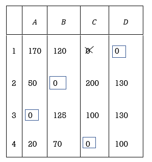
Optimal assignment and total sales are given below
Salesmen | Districts | Sales volume |
1 |  | 400 |
2 |  | 400 |
3 |  | 500 |
4 |  | 420 |
| 1720 units | |
Example 3:
Here are four machines W, X, Y and Z. Three jobs A, B and C are to be assigned to the 3 machines out of total 4 machines. The cost of assignment is given below. Find out the optimal assignment.
| W | X | Y | Z |
A | 18 | 24 | 28 | 32 |
B | 8 | 13 | 17 | 18 |
C | 10 | 15 | 19 | 22 |
Solution: 1. No. Of rows 
No. Of columns 
This is an unbalanced assignment problem as the number of rows are not equal to number of columns. Therefore, in order to make it a square matrix, add a dummy row (D) with zero cost elements. Thus, the modified matrix becomes
|  |  |  |  |
 | 18 | 24 | 28 | 32 |
 | 8 | 13 | 17 | 18 |
 | 10 | 15 | 19 | 22 |
 | 0 | 0 | 0 | 0 |
2. The reduced matrix after row operation is; (Column operation is not necessary as there is already one and, in each column,).
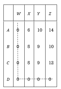
3. Minimum number of lines to connect all zeros is two (2) which is no. Of rows or columns. Therefore, proceed to next step.
4. Select the smallest element which is not covered by the lines and subtract it from all other elements which are not covered by the lines and add it at the intersection of two lines.
The resulting matrix is:
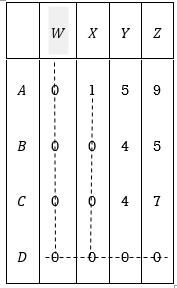
Minimum number of lines = 3 (less than the order of the matrix)
Therefore, repeat step 4, The result matrix is:

Transportation Model:
Transportation models address the issue of what happens to the effectiveness function when a number of origins (sources) are linked to a potentially varied number of destinations (jobs). The total movement from each origin and total movement to each destination are supplied, and it's up to you to figure out how to make the associations work within the totals constraints. Sources can be shared among the jobs in such situations, or jobs can be completed using a combination of sources. The fact that sources and jobs must be stated in terms of only one type of unit is a distinguishing feature of transportation difficulties.
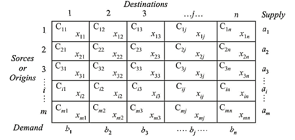
Assume you have m sources and n destinations. Let a; represent the number of supply units available at the source i(i = I, 2, 3,, m), and bf represent the number of demand units required at the destination j(i = I, 2, 3,..., n). Let  stand for the unit transportation cost of moving units from source i to destination j. The goal is to figure out how many units need to be transported from source I to destination J while keeping the total transportation cost to a minimum. Furthermore, supply constraints at the sources and demand needs at the destinations must be met precisely.
If  is the number of units shipped from source i to destination j, then the equivalent linear programming model will be
Find  in order to
Minimize 
Subject to


Where 
The two sets of constraints will be consistent ie the system will be in balance if

Exampe:1:
A dairy firm has three plants located in a state. Daily milk production at each plant is as follows:
Plant 1= 6 million litres, plant 2 =1 million litres, and plant 3 .=10 million litres.
Each day the firm must fulfil the needs of its four distribution centres. Milk requirement at each centre is as follows:
Distribution centre 1=7 million litres, distribution centre 2 =5 million litres, distribution centre 3 =3 million litres, and distribution centre 4 =2 million litres.
Cost of shipping one million litres of milk from each plant to each distribution centre is given in the following table in hundreds of rupees
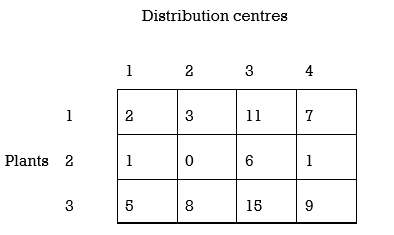
Solution:
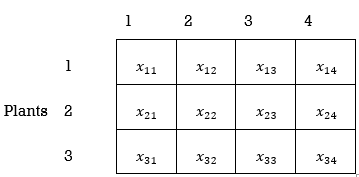


And
Step 2:
Feasible alternatives are sets of values of  , where
Step 3:
Objective is to minimize the cost of transportation.
i.e., minimize

Minimize

 (For milk plant 1)
 (For milk plant 2)
 (For milk plant 3)

 (For distribution 1)
 (For distribution 2)
 (For distribution 3)
 (For distribution 4)

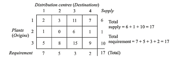
For Solution:
- Northwest Corner rule or Northwest corner method
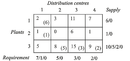
This rule may be stated as follows:
Start in the north-west (upper left) corner of the requirements table i.e., the transportation matrix framed in step I and compare the supply of plant 1 (call it S1) with the requirement of distribution centre 1 (call it D1).
If D1 < S1 i.e., if the amount required at D1 is less than the number of units available at S1, set x11 equal to D1, find the balance supply and demand and proceed to cell (I, 2) (i.e., proceed horizontally).
If D1 = S1, set x11 equal to D1, compute the balance supply and demand and proceed to cell (2, 2) (i.e., proceed diagonally).
If D1 > S1, set x11 equal to S1, compute the balance supply and demand and proceed to cell (2, 1) (i.e., proceed vertically).
Continue in this manner, step by step, away from the north-west corner until, finally, a value is reached in the south-east corner.
Thus, in the present example one proceeds as follows:
- Set x11 equal to 6, namely, the smaller of the amounts available at S1 (6) and that needed at D1 (7) and
- Proceed to cell (2, 1) (rule c). Compare the number of units available at S2 (namely 1) with the amount required at D1 (1) and accordingly set x21 = I.
- Proceed to cell (3, 2) (rule b). Now supply from plant S3 is 10 units while the demand for D2 is 5 units; accordingly set x32 equal to 5.
- Proceed to cell (3, 3) (rule a) and allocate 3 there.
- Proceed to cell (3, 4) (rule a) and allocate 2 there.
- It can be easily seen that the proposed solution is a feasible solution since all supply and demand constraints are fully satisfied.
The following points may be noted in connection with this method:
The quantities allocated are put in parenthesis and they represent the values of the corresponding decision variables. These cells are called basic or allocated or occupied or loaded cells. Cells without allocations are called non-basic or vacant or empty or unoccupied or unloaded cells. Values of the corresponding variables are all zero in these cells.
This method of allocation does not consider the transportation cost and, therefore, may not yield a good (most economical) initial solution. The transportation cost associated with this solution is

- Row minima method
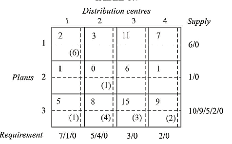
This method consists in allocating as much as possible in the lowest cost cell of the first row so that either the capacity of the first plant is exhausted, or the requirement atjth distribution centre is satisfied or both. In case of tie among the cost, select arbitrarily. Three cases arise:
if the capacity of the first plant is completely exhausted, cross off the first row and proceed to the second row.
if the requirement at jth distribution centre is satisfied, cross off the jth column and reconsider the first row with the remaining capacity.
if the capacity of the first plant as well as the requirement at Jth distribution centre are completely satisfied, cross off the row as well as the jth column and move down to the second row.
Continue the process for the resulting reduced transportation table until all the rim conditions
(Supply and requirement conditions) are satisfied.
In this problem, we first allocate to cell (1, 1) in the first row as it contains the minimum cost 2. We allocate min. (6, 7) = (6) in this cell. This exhausts the supply capacity of plant 1 and thus the first row is crossed off. The next allocation, in the resulting reduced matrix is made in cell (2, 2) of row 2 as it contains the minimum cost 0 in that row. We allocate min. (I, 5) = (I) in this cell. This exhausts the supply capacity of plant 2 and thus the second row is crossed off.
The next allocation, in the resulting reduced matrix is made in cell (3, I) of row 3 as it contains the minimum cost 5 in that row. We allocate min. (1, 10) = (1) in this cell. This exhausts the requirement condition of distribution centre I and hence the first column is crossed off. Proceeding in this way we allocate (4), (2) and (3) units to cells (3, 2), (3, 4) and (3, 3) till all the rim conditions are met with. The resulting matrix is shown.
The transportation cost associated with this solution is
 ,
,
Which is less than the cost associated with solution obtained by N-W corner method.
- Column minima method
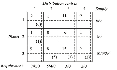
This method consists in allocating as much as possible in the lowest cost cell of the first column so that either the demand of the first distribution centre is satisfied or the capacity of the ith plant is exhausted or both. In case of tie among the lowest cost cells in the column, select arbitrarily. Three cases arise:
if the requirement of the first distribution centre is satisfied, cross off the first column and move right to the second column.
if the capacity of ith plant is satisfied, cross off ith row and reconsider the first column with the remaining requirement.
if the requirement of the first distribution centre as well as the capacity of the ith plant are completely satisfied, cross off the column as well as the ith row and move right to the second column.
Continue the process for the resulting reduced transportation table until all the rim conditions are satisfied.
In the given problem we allocate first to cell (2, 1) in the first column as it contains the minimum cost 1. We allocate min. (1, 7) = (1) in this cell. This exhausts the supply capacity of plant 2 and thus the second row is crossed off. The next allocation in the resulting reduced matrix is made in cell (1, 1) of column 1 as it contains the second lowest cost 2 in that column. We allocate min. (6, 6) = (6) in this cell. This exhausts the supply capacity of plant 1 as well as the requirement of distribution centre 1. Therefore, we cross off first row and first column and move on to the second column. Proceeding in this way we allocate (5), (3) and (2) to cells (3, 2), (3, 3) and (3, 4) till all the rim conditions are met with.
The transportation cost associated with this solution is

Which is same as the cost associated with solution obtained by N-W corner method
The steppingstone method:
Consider the matrix giving the initial feasible solution for the problem under consideration. Let us start with any arbitrary empty cell (a cell without allocation), say (3, 2) and allocate + 1 unit to this cell. As already discussed, to keep up the column 2 restriction, - 1 must be allocated to cell (1, 2) and to keep up the row 1 restriction, + 1 must be allocated to cell (1, 1) and consequently - 1 must be allocated to cell (3, 1); this is shown in the matrix below.
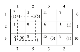
The net change in transportation cost as a result of this perturbation is called the evaluation of the empty cell in question.
∴ Evaluation of cell (3, 2)=₹100(8×1-5×1+2×1-5×1)=₹(0×100)=₹ 0
Thus, the total transportation cost increases by Rupee 0 for each unit allocated to cell (3, 2). Likewise, the net evaluation (also called opportunity cost) is calculated for every empty cell. For this the following simple procedure may be adopted.
Starting from the chosen empty cell, trace a path in the matrix consisting of a series of alternate horizontal and vertical lines. The path begins and terminates in the chosen cell. All other comers of the path lie in the cells for which allocations have been made. The path may skip over any number of occupied or vacant cells. Mark the comer of the path in the chosen vacant cell as positive and other comers of the path alternately -ve, +ve, -ve and so on. Allocate 1 unit to the chosen cell; subtract and add 1 unit from the cells at the comers of the path, maintaining the row and column requirements. The net change in the total cost resulting from this adjustment is called the evaluation of the chosen empty cell. Evaluations of the various empty cells (in hundreds of rupees) are:
Cell (1, 3) = c13 - c33 + c31 - c11 = 11 - 15 + 5 - 2 = - I, Cell (1, 4) = c14 - c34 + c31 - c11 = 7 - 9 + 5 - 2 = + I, Cell (2, I) = c21 - c24 + c34 - c31 = 1 - 1+ 9 - 5 = + 4,
Cell (2, 2) = c22 - c24 + c34 - c31 + c11 - c12 = 0 - 1 + 9 - 5 + 2 - 3 = + 2, Cell (2, 3) = c23 - c24 + c34 - c33 = 6 - I + 9 - 15 = - 1,
Cell (3, 2) = c32 - c31 + c11 - c12 = 8 - 5 + 2 - 3 = + 2.
If any cell evaluation is negative, the cost can be reduced so that the solution under consideration can be improved i.e., it is not optimal. On the other hand, if all cell evaluations are positive or zero, the solution in question will be optimal. Since evaluations of cells (1, 3) and (2, 3) are -ve, initial basic feasible solution given in table is not optimal.
Now in a transportation problem involving m rows and n columns, the total number of empty cells will be mn - (m + n - I) = (m - l)(n - 1). Therefore, there are (m - l)(n - 1) such cell evaluations which must be calculated and for large problems, the method can be quite inefficient. This method is named 'steppingstone' since only occupied cells or 'steppingstones' are used in the evaluation of vacant cells.
The Modified Distribution (MODI) Method or the u-v Method:
In the steppingstone method, a closed path is traced for each unoccupied cell. Cell evaluations are found and the cell with the most negative evaluation becomes the basic cell. In the modified distribution method, cell evaluations of all the unoccupied cells are calculated simultaneously and only one closed path for the most negative cell is traced. Thus, it provides considerable time saving over the steppingstone method.
- Determine an initial basic feasible solution using any one of the three methods given below:
Northwest Corner Rule
Matrix Minimum Method
- Determine the values of dual variables, ui and vj, using ui + vj = cij
- Compute the opportunity cost using Δij= cij – ( ui + vj ).
- Check the sign of each opportunity cost
The suggested solution is optimal if the opportunity costs of all empty cells are either positive or zero. However, if one or more vacant cells have a negative opportunity cost, the suggested approach is not ideal, and additional transportation cost savings are achievable.
- As the cell to be included in the next solution, choose the unoccupied cell with the smallest negative opportunity cost.
- For the unoccupied cell picked in the previous step, draw a closed path or loop. Please notice that in this course, the right-angle turn is only allowed at occupied cells and at the original vacant cell.
- At the vacant cells on the corner points of the closed path, alternate plus and minus signs, with a plus sign at the cell being examined.
- Calculate the maximum number of units that should be sent to this empty cell. The smallest value on the closed path with a negative position shows the maximum number of units that can be transported to the entering cell. Add this amount to all the cells marked with plus signs on the closed path's corner points and subtract it from the cells marked with minus signs. As a result, an unoccupied cell gets occupied.
- Repeat the process until you've found the best answer.
Example:
This method consists of the following sub steps
- Set up a cost matrix containing the unit costs associated with the cells for which allocations have been made. This matrix for the present example is

- Introduce dual variables corresponding to the supply and demand constraints. If there are m origins and n destinations, there will be m + n dual variables. Let ui (i = 1, 2, m) and vi (j = 1, 2, ... , n) be the dual variables corresponding to supply and demand constraints. Variables u; and vi are such that ui + vi = cij for all occupied cells.
Therefore, enter a set of numbers ui (i = I, 2, 3) along the left of the matrix and vi (j = I, 2, 3, 4) across the top of the matrix so that their sums equal the costs entered in sub step I.


Since number of dual variables are m + n (3 + 4 = 7 in the present problem) and number of allocations (in a non-degenerate solution) are m + n - 1 (3 + 4 - 1 = 6 in the present problem), one variable is assumed arbitrarily. Let Vi = 0. Therefore, from the above equations

The values of these dual variables satisfy the complementary slackness theorem which states that if primal constraints are equations, dual variables are unrestricted in sign
Therefore, the matrix may be written as
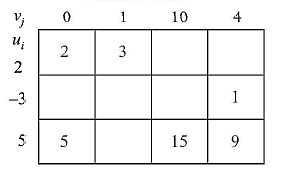
Now for any vacant (empty) cell,  is called the implicit cost, whereas
  is called the actual cost of the cell. The two costs are compared and
  are calculated for each empty cell. If all
  , then by the application of complementary slackness theorem it can be shown that the corresponding solution is optimum. If any
  , the solution is not optimal.
  is called the evaluation of the cell (i, j) or opportunity cost of cell (i, j), Thus we have the following three substeps:
Fill the vacant cells with the sums of ui and vj.
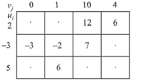
Subtract the cell values of the matrix of previous subset from the original cost matrix

Sub step 5: Signs of the values in the cell evaluation matrix indicate whether optimal solution has been obtained or not. The signs have the following significance:
- A negative value in an unoccupied cell indicates that a better solution can be obtained by allocating units to this cell.
- A positive value in an unoccupied cell indicates that a poorer solution will result by allocating units to the cell.
- A zero value in an unoccupied cell indicates that another solution of the same total value can be obtained by allocating units to this cell. In the present example since two cell evaluations are negative, it is possible to obtain a better solution by making these cells as basic cells
Iterate towards optimal solution:
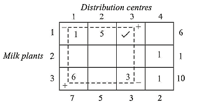

The total cost of transportation for this 2nd feasible solution is


Which is less than that for the first (starting) feasible solution 
Check for optimality:
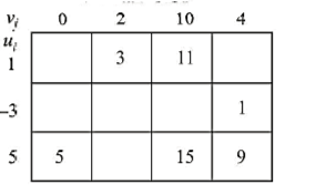
Thus 


Let 
Then 


Iterate towards an optimal solution:
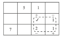

Test for optimality:
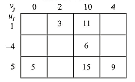
Substep 2: Enter a set of number  and
and  such that


Let 
Then 


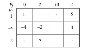


Therefore the optimal solution is
Milk plant | Distribution centre | No. Of units transported | Transportation cost/unit (₹) | Total Transportation cost (₹) |
1
2 3 | 2 3 3 1 3 4 | 5 1 1 7 1 2 | 300 1100 600 500 1500 900 | 1500 1100 600 3500 1500 1800 |
|
|
|
| ₹10,000 |
References:
1. Industrial Engineering and Production Management by Martand T Telsang S. Chand Publishing
2. Industrial Engineering and Production Management by M. Mahajan Dhanpat Rai& Co. (P) Limited
3. Industrial Engineering and Management by Ravi Shankar, Galgotia Publications Pvt Ltd
4. Production and Operations Management by Adam, B.E. & Ebert, R.J., PHI
5. Product Design and Manufacturing by Chitale A.V. And Gupta R.C., PHI