4.1 Beta and Gamma functions | unit 4 integral calculus

Back to Study material

MATHS I

UNIT 4

INTEGRAL CALCULUS

4.1 Beta and Gamma functions

Beta Function:

The Beta function is defined as

…(1)

Putting

i.e. Beta function is symmetric.

Another form of Beta function

Taking

This is the Euler’s integral of the first kind.

Gamma function:

The gamma function is defined as

This is the Euler’s Integral of the second kind.

Reduction formula for n:

Integration by parts

Where .

We have

2 =1.

1=1!

3=2.

2=2!

4=3.

3=3!

………………

d. 1=0!=1

Example1: Find the value of 1/2 ?

Let

Then

When

And then t=

Squaring both sides we get

where u and v is any variable in place of t.

Converting it in polar co-ordinates

Since

Relationship between Beta and Gamma functions

By the definition of gamma function we know that

Putting

Then

When then

then

Similarly

So, ()(

Converting into polar co-ordinates

Let

Also

Where

using definition

Example1: Compute

We have

Example2:Express in terms of gamma function

Given I =

Let

Then

Example3:Prove that

We know that

Putting

….(1)

Again putting

Let

When

Or ….(2)

From (1) and (2) we get

4.2 R.M.S value

The RMS value of a set of values (or a continuous-time waveform) is the square root of the arithmetic mean of the squares of the values, or the square of the function that defines the continuous waveform. In physics, the RMS current value can also be defined as the "value of the direct current that dissipates the same power in a resistor."

In the case of a set of n values , the RMS is

x RMS = 1 n ( x 1 2 + x 2 2 + ⋯

The corresponding formula for a continuous function (or waveform) f(t) defined over the interval $T_{1}\leq t\leq T_{2}$ is

f RMS = 1 T 2 −

and the RMS for a function over all time is

f RMS = lim T →

The RMS over all time of a periodic function is equal to the RMS of one period of the function. The RMS value of a continuous function or signal can be approximated by taking the RMS of a sample consisting of equally spaced observations. Additionally, the RMS value of various waveforms can also be determined without calculus, as shown by Cartwright.[4]

In the case of the RMS statistic of a random process, the expected value is used instead of the mean.

4.3 Differentiation of definite integrals

Example 1:

Solve the following

Solution:

= (0+1)-

= 1+

Example 2:

solve the integral

Solution:

Given,

4.4 (Leibnitz’s Rule)

Leibniz Integral Formula

Example 1:

Solve the following by using Leibniz Rule

Differentiate

Solution:

Using,

Example 2:

Solve the following

Solution:

And Hence,

To get rid of the constant C , notice that I(1)=0, so

Therefore,

4.5 Tracing of Curves (Cartesian, Standard Parametric and Polar Curves)

Tracing of Cartesian curves

The following rules will help in tracing a Cartesian curve.

Rule 1: Symmetry

(a) Symmetry about X-axis: If the equation of curve containing all even power terms in ‘y’ then the curve is symmetric about X-axis.

(b)Symmetry about Y-axis: If the equation of curve containing all even power terms in ‘x’ then the curve is symmetric about Y-axis {n \choose k}f^{(n-k

(C) Symmetry about both X and Y axes: If the equation of curve containing all even power terms in ‘x’ and ‘y’ then the curve is symmetric about both axes.

(d) Symmetry in opposite quadrants: If the equation of curve remains unchanged when x and y are replaced by –x and –y respectively then the curve is symmetric in opposite quadrants.

(e) Symmetry about the line :If the equation of curve remains unchanged when x is replaced by y and y is replaced by x then the curve is symmetric about the line y=x.

(f) Symmetry about the line :If the equation remains unchanged when x is replaced by -y and y is replaced by - x then the curve is symmetric about the line y=-x.

Rule 2: Points of intersection

(a) Origin: If the equation of curve does not contain any absolute constant then the curve passes through the origin.

(b) Intersection with the co-ordinate axes:

Intersection with X-axis: put y=0 in the given equation and find the value of x.

Intersection with Y-axis: put x = 0 in the given equation and find the value of y.

Rule 3:Tangents

(a) Origin:If the curve passes through origin then the equations of the tangent at origin can be obtained by equating the lowest degree terms taken together to zero.

(b) Other points:Tofind nature of tangent at any point find at that point.

Case 1: If then tangent is parallel to X-axis.

Case 2: If then tangent is parallel to Y-axis.

Case 3: If then tangent makes acute angle with X-axis.

Case 4: If then tangent makes obtuse angle with X-axis.

Rule 4:Asymptotes:

(a) Parallel to X-axis: Asymptotes parallel to X-axis are obtained by equating the coefficient of highest degree term in x to zero.

(b) Parallel to Y-axis: Asymptotes parallel to Y-axis are obtained by equating the coefficient of highest degree term in y to zero.

Method 1: Let y=mx+c be the asymptote. The point of intersection with the curve f(x, y)=0 are given by f(x, mx+c)=0. Equate to zero the coefficients of two successive highest power of ‘x’, giving equations to determine m & c.

Method 2:

Let y= mx+c be the equation of asymptote.
Find
by putting x=1 and y=m in the highest degree (n) terms of the equation.
Similarly find
.
Solve
=0 to determine m.
Find ‘c’ by the formula
.
If the roots of m are equal, then find ‘c’ by
.

Rule 5:Special points on the curve:Find out such points on the curve whose presence can be easily detected.

Rule 6:Region of absence of the curve: Findthe values of x(or y) where y(or x) becomes imaginary, then the curve does not exists in that region.

Q1. Trace the following curves

(i)

Solution:

- - - - - - - - - - - - - - - (1)

We check the following points for tracing of the above curve.

1. Symmetry:Since the power of y is even.

The curve is symmetry about x-axis.

No any other symmetry.

2. Origin:

Since there is no constant term in the given equation.

The curve passes through origin.

(i) Tangent at origin is given by

(ii) Nature of origin:

Since there is only one common tangent at origin.

Origin is cusp.

(iii) Intersection with coordinate axes:

Put in (1), we have.

Hence curve meets coordinate axes only at origin.

3. Asymptotes:

(i) Asymptotes parallel to x-axis:

Equating the coefficient of highest power of x, we obtain the asymptotes parallel to x-axis. Here highest power of x is and whose coefficient is 1 cannot equate to zero. Hence no asymptotes parallel to x-axis.

(ii) Asymptotes parallel to y-axis:

Equating the coefficient of highest power of y, we obtain the asymptotes parallel to y-axis. Here highest power of y is and whose coefficient is. Hence the asymptotes parallel to y-axis is

(iii) Oblique asymptotes:

Asymptotes not parallel to x and y axes are called oblique asymptotes.

Here since parallel asymptotes are present, so no oblique asymptotes.

4. Region:

From (1), we have

From the above expression, it is clear that

(i) If x is negative, then y will be imaginary. So, there is no part of the curve for which x is negative i.e. left hand side of y-axis.

(ii) If, then y will be imaginary. So, there is no part of the curve right hand side of the line.

Hence the approximate shape of the curve is as follows:

TRACING OF POLAR CURVES

The following rules will help in tracing a Polar curve.

Rule 1:Symmetry

(a) Symmetry about pole: If the equation of the curve remains unchanged by replacing then curve is symmetric to the pole.

(b) Symmetry about initial line: If the equation of the curve remains unchanged by replacing, then curve is symmetric about the initial line.

(c)Symmetry about :

1. If the equation of the curve remains unchanged by replacing

and, then curve is symmetric about the line .

2. If the equation of the curve remains unchanged by replacing

then curve is symmetric about the line .

Rule 2:Pole: If for some value of, r becomes zero then the pole will lie on the curve.

Rule 3:Tangents: To find tangents at the pole, put r = 0 in the equation, the values of gives the tangent at the pole.

Rule 4: Angle between radius vector and tangent :

Use the formula and find and also the points where

Rule 5: Form the table showing values of r for some values of

Rule 6: Find the region of absence of the curve.

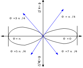
Q1. Trace the following curve:

Solution: We check the following points for tracing of the above curve

Limit: -
i. e. the curve lies between
.
Symmetry:

(i) About the Pole:

If we replace by, then the equation of the curve is remains unchanged.

The curve is symmetry about pole.

(ii) About initial line :-

If we replace by, then the equation of the curve is remains unchanged.

The curve is symmetry about the initial line.

(iii) About the line perpendicular to the initial line at pole or about the line:-

If we replace byand by, then the equation of the curve is remains unchanged.

The curve is symmetry about the line perpendicular to the initial line at pole or about the line.

3. Pole:

(i) For.

Hence the curve passes through the pole.

(ii) Tangent at Pole: If we put , then we get the tangent at pole.

Putting in (1), we have

4. Tangent:

5. Asymptotes:No asymptotes.

6. Table values:

It is clear that at, and the tangent is perpendicular to the initial line at and. Again at. Hence there is no part of the curve between. Also, the curve is symmetry about pole, initial line and the line perpendicular to initial line. Hence the approximate shape of the curve is as follows:

TRACING OF ROSE CURVES .

Rule 1: No. of loops:

If n is odd, then number of loops in the curve = n.
If n is even, then number of loops in the curve = 2n.

Rule 2: Symmetry

(a) Symmetry about initial line: If the equation of the curve remains unchanged by replacing, then the curve is symmetric about the initial line

(b) Symmetry about the line :

1. If the equation of the curve remains unchanged by replacing

and, then curve is symmetric about the line .

3. If the equation of the curve remains unchanged by replacing

then curve is symmetric about the line .

Rule 3:Pole:Find in particular values of, which give r = 0.

Rule 4:Tangents: To find tangents at the pole, put r =0 in the equation, the values of gives

the tangent at the pole.

Rule 5:Angle between radius vector and tangent :

Use the formula and find and also the points where

Rule 6:Form the table showing values of r for some values of

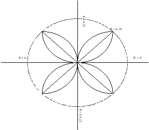
Q1. Trace the following curve:

Solution: We check the following points for tracing of the above curve

Limit:
i.e. total curve will lie inside the circle of radius ‘a’.
No. of loops: The curve contains 4 loops because
is even.
Symmetry:

(i) About the line perpendicular to initial line i.e. the line:-

If we replace by and bythen the equation of the curve is remains unchanged.

The curve is symmetry about the line.

Pole:

(i) For .

Hence the curve passes through the pole.

(ii) Tangent at pole: If we put , then we get the tangent at pole.

Putting in (1), we have

4. Asymptotes:No asymptotes.

5. Table values:


	0		0		0		0

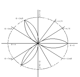
It is clear that for, the value of r is zero therefore these are tangents at pole and for the value of r is maximum i.e. ‘a’. Hence, we get four loops at those points. Hence the approximate shape of the curve is as follows.

Q. 2 Trace the following curve:

Solution: We check the following points for tracing of the above curve

Limit:
i.e. total curve will lie inside the circle of radius ‘a’.
No. of loops:The curve contains 3 loops because
is odd.
Symmetry:

(i) About initial line :-

If we replace by, then the equation of the curve is remains unchanged.

The curve is symmetry about the initial line.

4. Pole:

(i) For

Hence the curve passes through the pole.

(ii) Tangent at pole: If we put , then we get the tangent at pole.

Putting in (1), we have

5. Asymptotes:No asymptotes.

6. Table values:


			0		0		0	0

It is clear that for, the value of r is zero therefore these are tangents at pole and for the value of r is maximum i.e. ‘a’. Hence we get three loops at those points. Hence the approximate shape of the curve is as follows.

Reference Books:

1. A text book of Applied Mathematics Volume I and II by J.N. Wartikar and P.N. Wartikar

2. Higher Engineering Mathematics by Dr. B. S. Grewal

3. Advanced Engineering Mathematics by H. K. Dass

4. Advanced Engineering Mathematics by Erwins Kreyszig

Sign Up

Index

Notes

Highlighted

Underlined

Browse by Topics

Notes

Highlighted

Underlined