Unit-1
Partial differentiation and its Applications
First order partial differentiation-
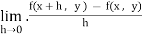
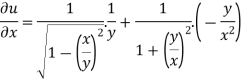
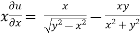
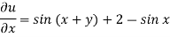
Let f(x, y) be a function of two variables. Then the partial derivative of this function with respect to x can be written as  and defined as follows:
 =
= 
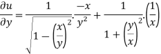
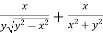
Now the partial derivative of f with respect to f can be written as  and defined as follows:
 =
= 
Note: a. While calculating partial derivatives treat all independent variables, other than the variable with respect to which we are differentiating , as constant.
b. We apply all differentiation rules.
Higher order partial differentiation-
Let f(x , y) be a function of two variables. Then its second-order partial derivatives, third order partial derivatives and so on are referred as higher order partial derivatives.
These are second order four partial derivatives:
(a)  =
= 
(b)  =
= 
(c)  =
= 
(d)  =
= 
b and c are known as mixed partial derivatives.
Similarly we can find the other higher order derivatives.
Example-1: -Calculate  and
and  for the following function
f(x , y) = 3x³-5y²+2xy-8x+4y-20
Sol. To calculate  treat the variable y as a constant, then differentiate f(x,y) with respect to x by using differentiation rules,
 =
=  [3x³-5y²+2xy-8x+4y-20]
=  3x³] -
  5y²] +
  [2xy] -
 8x] +
8x] + 4y] -
4y] -  20]
20]
= 9x² - 0 + 2y – 8 + 0 – 0
= 9x² + 2y – 8
Similarly partial derivative of f(x,y) with respect to y is:
 =
=  [3x³-5y²+2xy-8x+4y-20]
=  3x³] -
  5y²] +
  [2xy] -
 8x] +
8x] + 4y] -
4y] -  20]
20]
= 0 – 10y + 2x – 0 + 4 – 0
= 2x – 10y +4.
Example-2: Calculate  and
and  for the following function
f( x, y) = sin(y²x + 5x – 8)
Sol. To calculate  treat the variable y as a constant, then differentiate f(x,y) with respect to x by using differentiation rules,
 [sin(y²x + 5x – 8)]
= cos(y²x + 5x – 8) (y²x + 5x – 8)
= (y² + 50)cos(y²x + 5x – 8)
Similarly partial derivative of f(x,y) with respect to y is,
 [sin(y²x + 5x – 8)]
= cos(y²x + 5x – 8) (y²x + 5x – 8)
= 2xycos(y²x + 5x – 8)
Example-3: Obtain all the second order partial derivative of the function:
f( x, y) = ( x³y² - xy⁵)
Sol. 3x²y² - y⁵,
  2x³y – 5xy⁴,
 =
=  = 6xy²
 =
=  2x³ - 20xy³
 =
=  = 6x²y – 5y⁴
 =
=  = 6x²y - 5y⁴
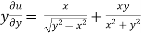
Example-4: Find

Sol. First we will differentiate partially with respect to r,

Now differentiate partially with respect to θ, we get

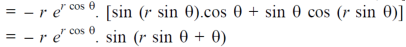
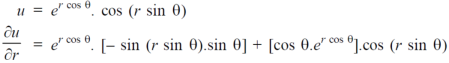
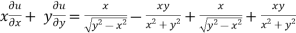
Example-5: if,

Then find.

Sol-

Example-6: if  , then show that-
Sol. Here we have,
u =  …………………..(1)
Now partially differentiate eq.(1) w.r to x and y , we get
= 
Or
 ………………..(2)
And now,
= 
 ………………….(3)
Adding eq. (1) and (3) , we get
 = 0
= 0
Hence proved.
Homogeneous function - A function f(x,y) is said to be homogeneous of degree n if,
f(kx, ky) = kⁿf(x, y)
Here, the power of k is called the degree of homogeneity.
Or
A function f(x,y) is said to be a homogenous function in which the power of each term is the same.
Example:
1. The function-
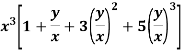
Is a homogeneous function of order 3
Euler’s theorem
Statement – if u = f(x, y) be a homogeneous function in x and y of degree n , then
x + y
+ y  = nu
= nu
Proof: Here u is a homogeneous function of degree n,
u = xⁿ f(y/x) ----------------(1)
Partially differentiate equation (1) with respect to x,
 = n
= n f(y/x) + xⁿ f’(y/x).(
 )
)
Now multiplying by x on both sides, we get
x = n
= n f(y/x) + xⁿ f’(y/x).(
 ) ---------- (2)
Again partially differentiate equation (1) with respect to y,
 = xⁿ f’(y/x).
Now multiplying by y on both sides,
y  = xⁿ f’(y/x).
 ---------------(3)
By adding equation (2) and (3),
x y
y  = n
= n f(y/x) + + xⁿ f’(y/x).(
 ) + xⁿ f’(y/x).
x y
y  = n
= n f(y/x)
Here u = f( x, y) is homogeneous function, then - u =  f(y/x)
Put the value of u in equation (4),
x y
y  = nu
= nu
Which is the Euler’s theorem.
Let’s understand Eulers’s theorem by some examples:
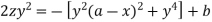
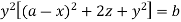
Example1-If u = x²(y-x) + y²(x-y), then show that  -2 (x – y)²
Solution - here, u = x²(y-x) + y²(x-y)
u = x²y - x³ + xy² - y³,
Now differentiate u partially with respect to x and y respectively,
 = 2xy – 3x² + y² --------- (1)
 = x² + 2xy – 3y² ---------- (2)
Now adding equation (1) and (2), we get
 = -2x² - 2y² + 4xy
= -2 (x² + y² - 2xy)
= -2 (x – y)²
Example2- If u = xy + sin(xy), show that  =
=  .
.
Solution – u = xy + sin(xy)
 = y+ ycos(xy)
 = x+ xcos(xy)
 x (- sin(xy).(y)) + cos(xy)
= 1 – xysin(xy) + cos(xy) -------------- (1)
 1 + cos(xy) + y(-sin(xy) x)
= 1 – xysin(xy) + cos(xy) -----------------(2)
From equation (1) and (2),
 =
= 
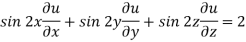
Example-3: If u(x,y,z) = log( tan x + tan y + tan z) , then prove that ,
Sol. Here we have,
u(x,y,z) = log( tan x + tan y + tan z) ………………..(1)
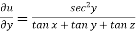
Diff. Eq.(1) w.r.t. x , partially , we get
 ……………..(2)
Diff. Eq.(1) w.r.t. y , partially , we get
 ………………(3)
Diff. Eq.(1) w.r.t. z , partially , we get
 ……………………(4)
Now multiply eq. 2 , 3 , 4 by sin 2x , sin 2y , sin 2z respectively and adding , in order to get the final result,
We get,

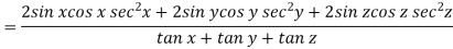
= 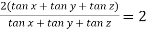
So that,
 hence proved.
Implicit differentiation-
Let f(x,y) = 0
Where y = ∅(x)
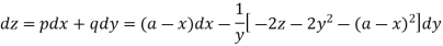
By the chain rule , with x = x and y = ∅(x), we get
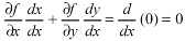

Here we assume that y is a differentiable funtion of x.
Example-1: if ∅ is a differentiable function such that y = ∅(x) satisfies the equation
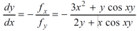
x³ + y³ +sin xy = 0 then find  .
.
Sol. Suppose f(x,y) = x³ + y³ +sin xy
Then ,
fᵡ= 3x² + y cosxy
Fy = 2y + x cosxy
So ,
Example-2:
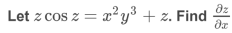
Sol. Take partial derivative on both side w.r. t. x , treat y as constant
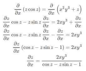
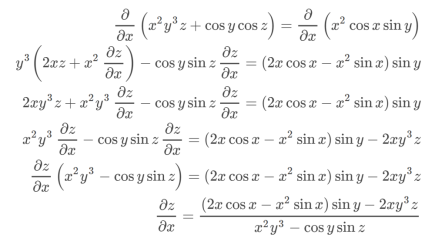
Example-3: if x²y³ + cos y cosz = x²cos x sin y, then find 
Sol. Differentiate partially w.r.t. x and treat y as constant,
When we measure the rate of change of the dependent variable owing to any change in a variable on which it depends, when none of the variable is assumed to be constant.
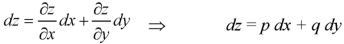
Let the function, u = f( x, y), such that x = g(t) , y = h(t)
ᵡ Then we can write,
 =
= 
= 
This is the total derivative of u with respect to t.
If w = f (x, y) has continuous partial variables fxand fyand if x = x (t), y = y (t) are
Differentiable functions of t, then the composite function w = f (x (t), y (t)) is a
Differentiable function of t.
In this case, we get,
 fx(x (t), y (t)) x’(t)+ fy(x(t), y (t)) y’(t).
Example-:1 let q = 4x + 3y and x = t³ + t² + 1 , y = t³ - t² - t
Then find  .
.
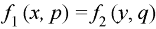
Sol. : . =
. = 
Where, f1 =  , f2 =
In this example f1 = 4 , f2 = 3
Also,  3t² + 2t ,
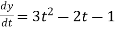
 4(3t² + 2t) + 3(
= 21t² + 2t – 3
Example-2: Find  if u = x³y⁴ where x = t³ and y = t².
Sol. As we know that by definition,  =
= 
 3x²y⁴3t² + 4x³y³2t = 17t¹⁶.
Example-3: if w = x² + y – z + sintand x + y = t, find
(a)  y,z
y,z
(b)  t, z
t, z
Sol. With x, y, z independent, we have
t = x + y, w = x²+ y - z + sin (x + y).
Therefore,
 y,z = 2x + cos(x+y)
 (x+y)
(x+y)
= 2x + cos (x + y)
With x, t, z independent, we have
Y = t-x, w= x² + (t-x) + sin t
Thus t, z = 2x - 1
Example-4: If u = u( y – z , z - x , x – y) then prove that  = 0
= 0
Sol. Let,

Then,

By adding all these equations we get,
 = 0 hence proved.
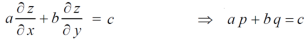
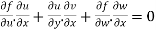
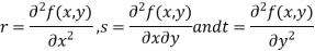
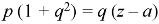
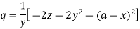
Example-5: if φ( cx – az , cy – bz) = 0 then show that ap + bq = c
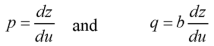
Where p =  q =
q = 
Sol. We have,
φ( cx – az , cy – bz) = 0
φ( r , s) = 0
Where,
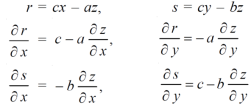
We know that,

Again we do,
By adding the two results, we get
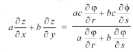
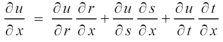
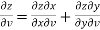
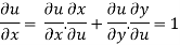
Example-6: If z is the function of x and y , and x =  , y =
, y =  , then prove that,
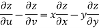
Sol. Here , it is given that, z is the function of x and y & x , y are the functions of u and v.
So that,
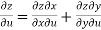 ……………….(1)
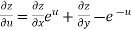
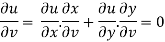
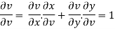
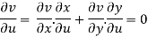
And,
 ………………..(2)
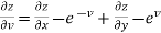
Also there is,
x =  and y =
  ,
,
Now,
 ,
,  ,
,  ,
, 
From equation(1) , we get
 ……………….(3)
And from eq. (2) , we get
 …………..(4)
Subtracting eq. (4) from (3), we get
 =
=  )
) – (
– (
= x
Hence proved.
If u and v are functions of the two independent variables x and y , then the determinant,

Is known as the jacobian of u and v with respect to x and y, and it can be written as,
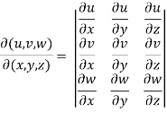
Suppose there are three functions u , v and w of three independent variables x , y and z then,
The Jacobian can be defined as,
Important properties of the Jacobians-
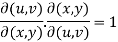
Property-1-
If u and v are the functions of x and y , then
Proof- Suppose u = u(x,y) and v = v(x,y) , so that u and v are the functions of x and y,
Now,
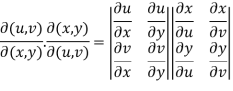
Interchange the rows and columns of the second determinant, we get
= 
=  ………….(1)
Differentiate u = u(x,y) and v= v(x,y) partially w.r.t. u and v, we get
Putting these values in eq.(1) , we get
 hence proved.
Property-2:
Suppose u and v are the functions of r and s, where r,s are the fuctions of x , y, then,
Proof:  =
= 
Interchange the rows and columns in second determinant
We get,
= 
= 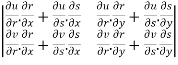
=  =
= 
Similarly we can prove for three variables.
Property-3
If u,v,w are the functions of three independent variables x,y,z are not independent , then,

Proof: here u,v,w are independent , then f(u,v,w) = 0 ……………….(1)
Differentiate (1), w.r.t. x, y and z , we get
 …………(2)
 ………………(3)
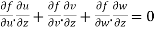 ………………..(4)
Eliminate  from 2,3,4 , we get

Interchanging rows and columns , we get
 = 0
= 0
So that,

Example-1: If x = r sin , y = r sin
 , z = r cos
 , then show that
 sin
sin also find
Sol. We know that,
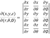
= 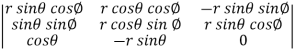
= 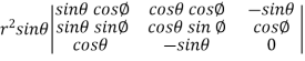
= 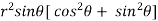 ( on solving the determinant)
= 
Now using first property of Jacobians, we get
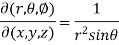
Example-2: If u = x + y + z ,uv = y + z , uvw = z , find 
Sol. Here we have,
x = u – uv = u(1-v)
y = uv – uvw = uv( 1- w)
And z = uvw
So that,

=
Apply 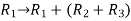
=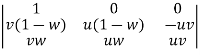
Now we get,
= u²v(1-w) + u²vw
= u²v
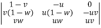
Example-3: If u = xyz , v = x² + y² + z² and w = x + y + z, then find J = 
Sol. Here u ,v and w are explicitly given , so that first we calculate
J’ = 
J’ =  =
= 
= yz(2y-2z) – zx(2x – 2z) + xy (2x – 2y) = 2[yz(y-z)-zx(x-z)+xy(x-y)]
= 2[x²y - x²z - xy² + xz² + y²z - yz²]
= 2[x²(y-z) - x(y² - z²) + yz (y – z)]
= 2(y – z)(z – x)(y – x)
= -2(x – y)(y – z)(z – x)
By the property,
JJ’ = 1
J = 
Taylor’s Theorem-
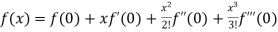
If f(x + h) is a function of h which can be expanded in the ascending powers of h and is differentiable by any number of times with respect to h, then-
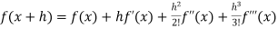 + …….+
  + ……..
Which is called Taylor’s theorem.
If we put x = a, we get-
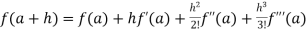 + …….+
  + …….. (1)
Maclaurin’s Theorem-
If we put a = 0 and h = x then equation(1) becomes-
 + …….
+ …….
Which is called Maclaurin’s theorem.
Note – if we put h = x - a then there will be the expansion of F(x) in powers of (x – a)
We get-
 + …….
+ …….
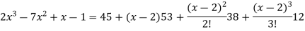
Example-1: Express the polynomial 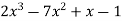 in powers of (x-2).
Sol. Here we have,
f(x) = 
Differentiating the function w.r.t.x-
f’(x) = 
f’’(x) = 12x + 14
f’’’(x) = 12
f’’’’(x)=0
Now using Taylor’s theorem-
 + ……. (1)
Here we have, a = 2,
Put x = 2 in the derivatives of f(x), we get-
f(2) = 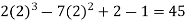
f’(2) = 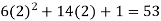
f’’(2) = 12(2)+14 = 38
f’’’(2) = 12 and f’’’’(2) = 0
Now put a = 2 and substitute the above values in equation(1), we get-

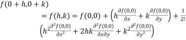
Taylor’s theorem for functions of two variables-
Suppose f(x , y) be a function of two independent variables x and y. Then,
 + ……………
Maclaurin’s series is the special case of Taylor’s series-
When we put a = 0 and b = 0 (about origin) in Taylor’s series, we get-
 + ……………
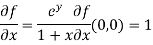
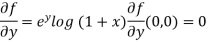
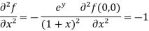
Example-2: Expand f(x , y) =  in powers of x and y about origin.
Sol. Here we have the function-
f(x , y) = 
Here , a = 0 and b = 0 then
f(0 , 0) = 
Now we will find partial derivatives of the function-

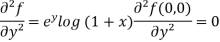
Now using Taylor’s theorem-
 +………
+………
Suppose h = x and k = y , we get
 +…….
+…….
=  +……….
+……….
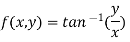
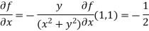
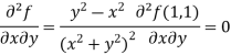
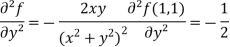
Example-3: Find the Taylor’s expansion of  about (1 , 1) up to second degree term.
Sol. We have,
At (1 , 1)


Now by using Taylor’s theorem-
 ……
……
Suppose 1 + h = x then h = x – 1
1 + k = y then k = y - 1
 ……
……
 =
= 
 ……..
……..
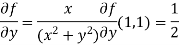
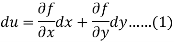
Let u = f(x , y) then the total differential of u which is denoted by du and defined as-
If  and
and  are increments in x and y respectively then the total increment
  in u is given by,

Or

But

Now from first equation-

By using equation (3) in (2) we get the approximation formula-
 .......... (iv)
We obtain the approximate value of the function by (4)
Hence

And
Example: Calculate the percentage increase in the pressure p corresponding to a reduction
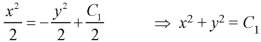
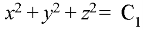
Of 1/2 % in the volume V, if the p and V are related by  = C, where C is a constant.
Sol.
Here we have-
 = C
= C
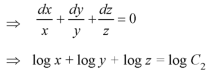
Taking log on both sides,
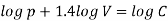
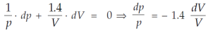
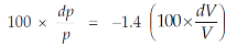
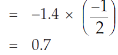
Hence increase in the pressure p = 0.7 percent
Example: Find the approximate value of –
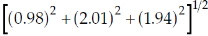
Sol.
Let
Then-

And
Now

Let


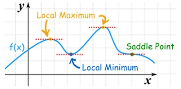
Maxima and minima of function of two variables-
As we know that the value of a function at maximum point is called maximum value of a function. Similarly the value of a function at minimum point is called minimum value of a function.
The maxima and minima of a function is an extreme biggest and extreme smallest point of a function in a given range (interval) or entire region. Pierre de Fermat was the first mathematician to discover general method for calculating maxima and minima of a function. The maxima and minima are complement of each other.
Maxima and Minima of a function of one variables
If f(x) is a single valued function defined in a region R then
Maxima is a maximum point  if and only if
Minima is a minimum point  if and only if


Maxima and Minima of a function of two independent variables
Let  be a defined function of two independent variables.
Then the point  is said to be a maximum point of
  if
if
Or  =
= 
For all positive and negative values of h and k.
Similarly the point  is said to be a minimum point of
  if
if
Or  =
= 
For all positive and negative values of h and k.
Saddle point: Critical points of a function of two variables are those points at which both partial derivatives of the function are zero. A critical point of a function of a single variable is either a local maximum, a local minimum, or neither. With functions of two variables there is a fourth possibility - a saddle point.
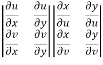
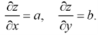
A point is a saddle point of a function of two variables if
![2 2 [ 2 ] 2
@f-= 0, @f--= 0, and @-f- @-f-- -@-f- < 0
@x @y @x2 @y2 @x @y](https://glossaread-contain.s3.ap-south-1.amazonaws.com/epub/1643032039_583525.png)
At the point.
Stationary Value
The value  is said to be a stationary value of
  if
if
i.e. the function is a stationary at (a , b).
Rule to find the maximum and minimum values of 
- Calculate
 .
. - Form and solve
 , we get the value of x and y let it be pairs of values
- Calculate the following values :
4. (a) If 
(b) If 
(c) If 
(d) If 
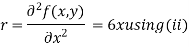
Example1 Find out the maxima and minima of the function

Given  …(i)
…(i)
Partially differentiating (i) with respect to x we get
 ….(ii)
Partially differentiating (i) with respect to y we get
 ….(iii)
Now, form the equations 
Using (ii) and (iii) we get


 using above two equations
Squaring both side we get

Or 
This show that 
Also we get 
Thus we get the pair of value as 
Now, we calculate
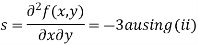

Putting above values in
At point (0,0) we get

So, the point (0,0) is a saddle point.
At point  we get

So the point  is the minimum point where
In case 

So the point  is the maximum point where
Example2 Find the maximum and minimum point of the function
Partially differentiating given equation with respect to and x and y then equate them to zero
On solving above we get 
Also 
Thus we get the pair of values (0,0), ( ,0) and (0,
Now, we calculate
At the point (0,0)
So function has saddle point at (0,0).
At the point (

So the function has maxima at this point ( .
.
At the point (0,

So the function has minima at this point (0, .
.
At the point (
So the function has an saddle point at (
Let  be a function of x, y, z which to be discussed for stationary value.
Let  be a relation in x, y, z
 for stationary values we have,

i.e.  … (1)
… (1)
Also from  we have
 … (2)
… (2)
Let ‘ ’ be undetermined multiplier then multiplying equation (2) by
  and adding in equation (1) we get,

 … (3)
… (3)
 … (4)
… (4)
 … (5)
… (5)
Solving equation (3), (4) (5) & we get values of x, y, z and  .
.
- Decompare a positive number ‘a’ in to three parts, so their product is maximum
Solution:
Let x, y, z be the three parts of ‘a’ then we get.
 … (1)
… (1)
Here we have to maximize the product
i.e. 
 By Lagrange’s undetermined multiplier, we get,

 … (2)
… (2)
 … (3)
… (3)
 … (4)
… (4)
i.e.
 … (2)’
 … (3)’
 … (4)
… (4)


And 


From (1)


Thus  .
.
Hence their maximum product is  .
.
2. Find the point on plane  nearest to the point (1, 1, 1) using Lagrange’s method of multipliers.
Solution:
Let  be the point on sphere
  which is nearest to the point
  . Then shortest distance.


 Let
Let 
Under the condition  … (1)
… (1)
 By method of Lagrange’s undetermined multipliers we have

 … (2)
… (2)

 … (3)
… (3)
i.e.  &
&

 … (4)
… (4)
From (2) we get 
From (3) we get 
From (4) we get 
 Equation (1) becomes

i.e. 


y = 2

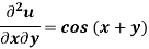
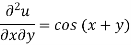
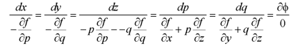
A differential equation involving partial derivatives with respect to more than one independent variable is called a partial differential equation.
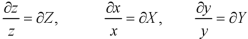
The independent variables will be denoted by x and y and the dependent variable by z. The partial differential coefficients are denoted as-
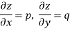
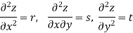
ORDER of a partial differential equation is the same as that of the order of the highest differential coefficient in it.
Classification of partial differential equation-
Suppose the equation is-
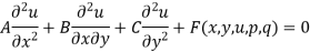
Here A, B, C are the constants of x and y, then the equation-
1. Elliptical- if 
2. Parabolic- if 
3. Hyperbolic- if if
Formation of partial differential equation-
Method of elimination of arbitrary constants-
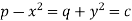
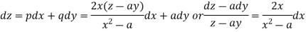
Example: Form a partial differential equation from-
Sol.
Here we have-

It contains two arbitrary constants a and c
Differentiate the equation with respect to p, we get-
Or
Now differentiate the equation with respect to q, we get-

Now eliminate ‘c’,
We get

Now put z-c in (1), we get-

Or

The second method we use is method of elimination of arbitrary function.
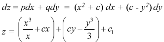
Solution of partial differential equation by direct partial Integration-
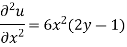
Example: Solve-
Sol.
Here we have-

Integrate w.r.t. x, we get-

Integrate w.r.t. x, we get-
Integrate w.r.t. y, we get-
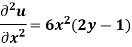
Example: Solve the differential equation-

Given the boundary condition that-
At x = 0, 
Sol.
Here we have-
On integrating partially with respect to x, we get-
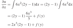
Here f(y) is an arbitrary constant.
Now form the boundary condition-
When x = 0,

Hence-

On integrating partially w.r.t.x, we get-
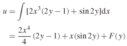
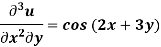
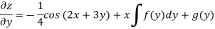
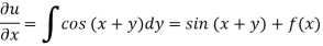
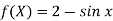
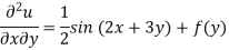
Example: Solve the differential equation-
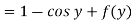
Given that  when y = 0, and u =
  when x = 0.
Sol.
We have-
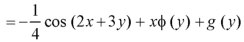
Integrating partially w.r.t. y, we get-
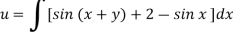
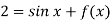
Now from the boundary conditions, 
Then-

From which,
It means,

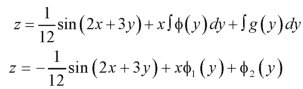
On integrating partially w.r.t. x givens-

From the boundary conditions, u =  when x = 0

From which-

Therefore the solution of the given equation is-

Solution of partial differential equation by direct partial Integration-
Example: Solve-

Sol.
Here we have-

Integrate w.r.t. x, we get-
Integrate w.r.t. x, we get-


Integrate w.r.t. y, we get-

Example: Solve the differential equation-
Given the boundary condition that-
At x = 0, 
Sol.
Here we have-

On integrating partially with respect to x, we get-

Here f(y) is an arbitrary constant.
Now form the boundary condition-
When x = 0,

Hence-

On integrating partially w.r.t.x, we get-

Example: Solve the differential equation-

Given that  when y = 0, and u =
  when x = 0.
Sol.
We have-

Integrating partially w.r.t. y, we get-

Now from the boundary conditions, 
Then-
From which,

It means,
On integrating partially w.r.t. x givens-


From the boundary conditions, u =  when x = 0


From which-
Therefore the solution of the given equation is-

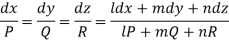
Lagrange’s linear equation in an equation of the type-

Here P, Q and R are the functions of x, y, z and p =  and q =
Working steps to solve-
Step-1: Write down the auxiliary equation-

Step-2: Solve the auxiliary equations-
Suppose the two solutions are- u =  and v =
Step-3: Then f(u, v) = 0 or u = ∅(v) is the required solution of

Method of multipliers-
Let the auxiliary equation be

L, m, n may be the constants of x, y, z then we have-
L, m, n are selected in a such a way that-
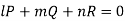
Thus
On solving this differential equation, if the solution is- u = 
Similarly, choose another set of multipliers  and if the second solution is v =
So that the required solution is f(u, v) = 0.
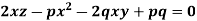
Example: Solve-
Sol.
We have-
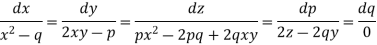
Then the auxiliary equations are-
Consider first two equations only-


On integrating
 …….. (2)
Now consider last two equations-


On integrating we get-
 …………… (3)
From equation (2) and (3)-
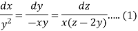
Example: Find the general solution of-
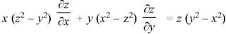
Sol. The auxiliary simultaneous equations are-
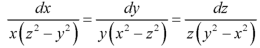 ……….. (1)
Using multipliers x, y, z we get-
Each term of (1) is equals to-

Xdx + ydy + zdz=0
On integrating-
 ………… (2)
Again equation (1) can be written as-

Or

 ………….. (3)
From (2) and (3), the general solution is-
Non-linear partial differential equations-
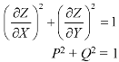
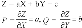
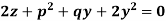
Type-1: Equation of the type f(p, q) = 0
Method-
Let the required solution is-
Z = ax + by + c …….. (1)
So that-
On putting these values in f(p, q) = 0
We get-
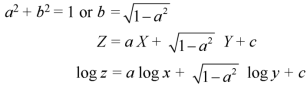
f(a, b) = 0
So from this, find the value of b in terms of a and put the value of b in (1). It will be the required solution.
Type-2: Equation of the type-
Z = px + qy + f(p, q)
Its solution will be-
Z = ax + by + f(a, b)
Type-3: Equation of the type f(z, p, q) = 0
Type-4: Equation of the type-
Method-
Let-


Example: Solve-
Sol.
This equation can be transformed as-


 ………. (1)
Let

Equation (1) can be written as-
 ………… (2)
Let the required solution be-
From (2) we have-
Example: Solve-
Sol.
Let u = x + by
So that-
Put these values of p and q in the given equation, we get-

Example: Solve-
Sol.
Let-
That means-

Put these values of p and q in
This is the general method for finding the complete integral of a non-linear partial differential equation.
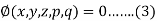
Let us consider the equation-
f(x, y, z , p, q) = 0 ………. (1)
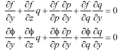
Since z depends on x and y, we have-

The main thing in Charpit’s method is to find the another relationship between the variables x, y, z and p. q.
And let the relation be-
Here on solving equation (1) and (2), we get the values of p and q.
When we substitute these values of p and q in (2), it becomes integrable.
To determine  , equation (1) and (3) are differentiated with respect to x and y.
We get, when we differentiate with respect to x,
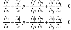
We get, when we differentiate with respect to y,
Eliminating  between the equations we get from differentiating for x, we get
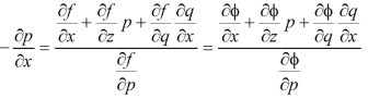
Or
 …………(4)
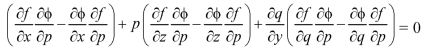
Eliminating  between the equations we get from differentiating for y, we get
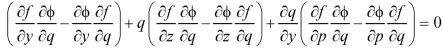 …………(5)
Adding (4) and (5) and keeping in view the relation on, the terms of the last brackets of (4) and (5) cancel. On rearranging, we get-

Or

This equation is the Lagrange’s linear equation of the first order with x, y, z, p, q as independent variables and equation (4) as dependent variable.
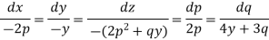
Its subsidiary equations are-
An integral of these equations involving p or q or both can be taken as the relation (3) which along with (1) will give the values of p and q to make (2) integrable.
Example: Solve-
Sol.
Let
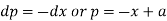
Charpit’s subsidiary equations are-
So that- dq = 0 or q = a
On putting q = a in (1) we get-
Such that-
Integrating

Or

Which is the required solution.
Example: Solve-
Sol.
Let

Charpit’s subsidiary equations are-
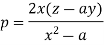
From the first and fourth ratios,
Substituting p = a – x in the given equation, we get-
So that-
Multiply both sides by  ,
,

Integrating-
Or
Which is the required solution.


