Unit-4

Multiple integrals

4.1. Multiple integrals: Double Integrals

Double integral –

Before studying about multiple integrals, first let’s go through the definition of definition of definite integrals for function of single variable.

As we know, the integral

Where is belongs to the limit a ≤ x ≤ b

This integral can be written as follows-

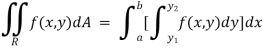
Now suppose we have a function f(x , y) of two variables x and y in two dimensional finite region R in xy-plane.

Then the double integration over region R can  be evaluated by two successive integration

Evaluation of double integrals-

If A is described as 

Then,

Let do some examples to understand more about double integration-

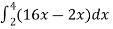
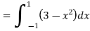
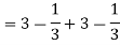
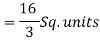
Example-1: Evaluate , where dA is the small area in xy-plane.

Sol.     Let ,     I = 

=

= 

= 

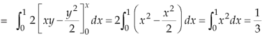
=    84 sq. Unit.

Which is the required area.

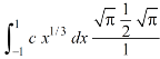
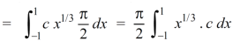
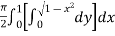
Example-2:  Evaluate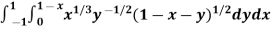

Sol. Let us suppose the integral is I,

I =

Put c = 1 – x in I, we get

I =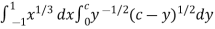

Suppose , y = ct

Then dy = c

Now we get,

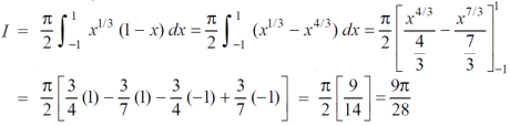
I =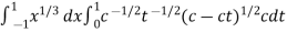

I =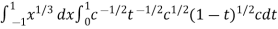

I =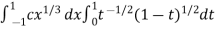

I =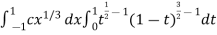

I  =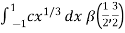

As we know that by beta function,

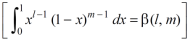
Which gives,

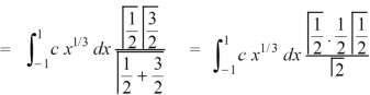
Now put the value of c, we get

Example-3:  Evaluate the following double integral,

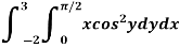
Sol.  Let ,

I =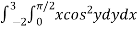 

On solving the integral, we get

Example-4: Evaluate-

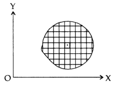
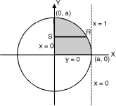
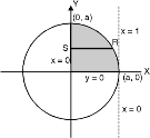
Where R is the quadrant of the circle .

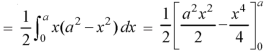
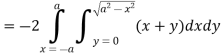
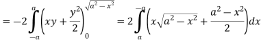
Sol.

Suppose the region of integration is the first quadrant of the circle OAB.

(

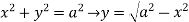
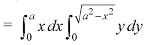
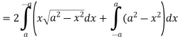
First we will integrate w.r.t. x then w.r.t. y-

The limits for y are 0 and and limits for x are 0 to a.

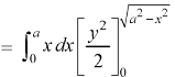
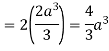
We get-

Evaluation of double integrals in polar coordinates-

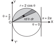
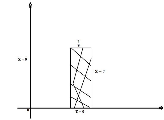
Example: Evaluate-

Sol.

Here we have-

Limits of y-

It represents the circle with centre (1, 0) and radius 1.

Lower limit of y is 0.

Region of integration is upper half circle.

Let convert the equation (1) into polar coordinates by putting-

X =  rcosθ and y =  r cosθ

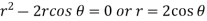
Limits of r are 0 to

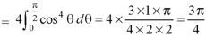
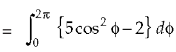
Limits of are 0 to π/2

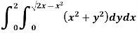
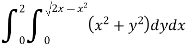
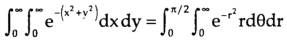
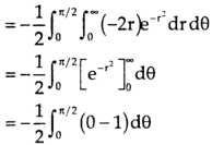
Example: Evaluate-

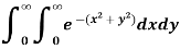
By changing into polar coordinates.

Sol.

We have

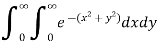
The limits of x and y are 0 to

Hence the region of integration is in the first quadrant,

The region is covered by the radius strip from r = 0 to r = ∞ and it starts from θ = 0 to θ = π/2

Hence the integral becomes-

4.2. Change of order of integration

Example-1 : Change the order of integration for the integral 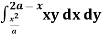 and evaluate the same with reversed order of integration.             

Soln. :  

Given,  

I = …(1)

In the given integration, limits are

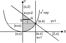
y=, y = 2a – x and x = 0,   x = a

The region bounded by x2 = ay, x + y = 2a    Fig.6.5

And x = 0, x = a is as shown in Fig. 6.5

Here we have to change order of Integration. Given the strip is vertical.

Now take horizontal strip SR.

To take total region, divide region into two parts by taking line y = a.  

1st Region:

Along strip, y constant and x varies from x = 0 to x = 2a – y. Slide strip IIelto  x-axis therefore y varies from y = a to y = 2a.

     I1 =dyxy dx …(2)

2nd Region:

Along strip, y constant and x varies from x = 0 to x = . Slide strip IIel to x-axis therefore x-varies from y = 0 to y = a.

   I2 =dyxy dx    …(3)

From Equation (1), (2) and (3),

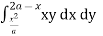   =  dyxy dx + dyxy dx

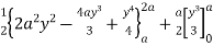
= +  y dy

=dy  + (ay) dy =  y (4a2 – 4ay + y2) dy +  ay2dy

=  (4a2 y – 4ay2 + y3) dy +   y2dy

= 

= +

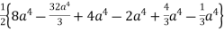=            a4

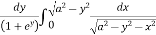
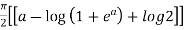
Example-2 : Evaluate

I =

Soln. :  

Given : I =     …(1)

In the given integration, limits are

x = 0, x = a,   y = 0,   y =

The bounded region is as shown in Fig. **.

In the given, strip is vertical. Now take horizontal strip SR. Along strip y constant and x varies from x = 0 to

x = . Slide strip IIel to X-axis therefore y varies from y = 0 to y = a.

   I=dy

=

Put  a2 – y2 = b2

 I=

=  =

= dy = dy

= 

=

= 

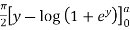
=  [∵ a = a loge]

  I = dy =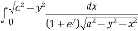 

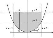
Example-3 : Express as single integral and evaluate dy dx + dy dx.

Soln: 

Given:

I  =  dy dx + dy dx 

I  =  I1 + I2

The limits of region of integration I1 are
x = – ; x =  and y = 0, y = 1 and I2 are x = – 1,
x = 1 and y = 1, y = 3.

The region of integration are as shown in Fig. 6.7

To consider the complete region take a vertical strip SR along the strip y varies from y = x2 to
y = 3 and x varies from x = –1 to x = 1. Fig. 6.7

I  =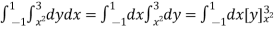

4.3. Triple integrals

Definition: Let f(x,y,z) be a function which is continuous at every point of the finite region (Volume V) of three dimensional space. Divide the region V into n sub regions of respective volumes. Let () be a point in the    sub region then the sum:

=

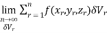
Is called triple integration of f(x, y, z) over the region V provided limit on R.H.S of above Equation exists.

Spherical Polar Coordinates

Where the integral is extended to all positive values of the variables subjected to the condition

Ex.1: Evaluate

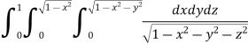
Solution : Let

I     =    

=    

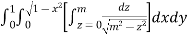
(Assuming m = )

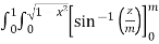= dxdy

=

=

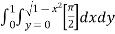
= dx

=  dx

= 

=

I =

Ex.2: Evaluate        Where V is annulus between the spheres 

And  ()

Solution:  It is convenient to transform the triple integral into spherical polar co-ordinate by putting

,                      ,   

,    dxdydz=sindrdd,   

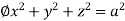and

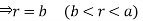
For the positive octant,  r  varies from  r =b to r =a  ,     varies from

And     varies from

I= 

= 8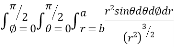

=8

=8

=8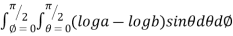

=8 log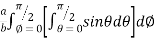

= 8 log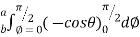

I= 8 log

I =  4 log

Ex.3: Evaluate

Solution:-

Ex.4:Evaluate

Solution:-

NOTES:

The volume of solid is given by

Volume =

In Spherical polar system 

In cylindrical polar system

Ex.1: Find Volume of the tetrahedron bounded by the co-ordinate’s planes and the plane

Solution: Volume =                                                 ………. (1)   

Put          ,  

From     equation (1) we have

V =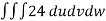

=24

=24           (u+v+w=1)  By Dirichlet’s theorem.

=24

=  ==  4

Volume =4

Ex.2:  Find volume common to the cylinders,  .

Solution:    For given cylinders,

,    .

Z varies from

Z=-to  z =

Y varies from

y= -to  y =

x varies from   x= -a to x = a

By symmetry,

Required volume= 8 (volume in the first octant)

=8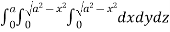

=8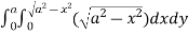

= 8dx

=8

=8

=8

Volume   =   16

Ex.3:  Evaluate   

1. Solution:-                  

Ex.4:

Ex.5: Evaluate

Solution:-   Put

4.4. Vector calculus: scalar and vector functions

Vector function-

Suppose be a function of a scalar variable t, then-

Here vector varies corresponding to the variation of a scalar variable t that its length and direction be known as value of t is given.

Any vector  can be expressed as-

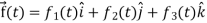
Here , , are the scalar functions of t.

Differentiation of a vector-

Note-

1. Velocity =

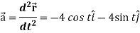
2. Acceleration =

Example: A particle is moving along the curve x = 4 cos t, y = 4 sin t, z = 6t. Then find the velocity and acceleration at time t = 0 and t = π/2.

And find the magnitudes of the velocity and acceleration at time t.

Sol. Suppose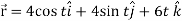

Now,

At t = 0	4
At t = π/2	-4
At t = 0	|v|=
At t = π/2	|v|=

Again acceleration-

Now-

At t = 0
At t = π/2
At t = 0	|a|=
At t = π/2	|a|=

Scalar point function-

If for each point P of a region R, there corresponds a scalar denoted by f(P), in that case f is called scalar point function of the region R.

Note-

Scalar field- this is a region in space such that for every point P in this region, the scalar function ‘f’ associates a scalar f(P).

Vector point function-

If for each point P of a region R, then there corresponds a vector then is called a vector point function for the region R.

Vector field-

Vector filed is a reason in space such that with every point P in the region, the vector function associates a vector (P).

Note-

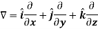
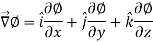
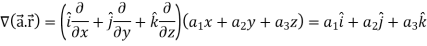
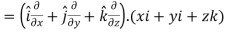
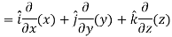
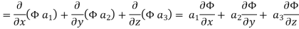
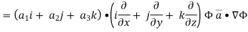
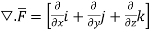
Del operator-

The del operated is defined as-

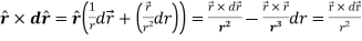
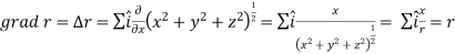
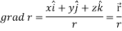
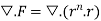
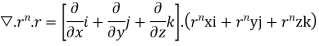
Example: show that  where

Sol. Here it is given-

=

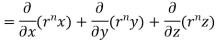
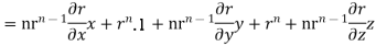
Therefore-

Note-

Hence proved.

4.5. Gradient, divergence and curl

Gradient of a scalar field

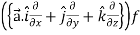
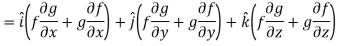
Suppose f(x, y, z) be the scalar function and it is continuously differentiable then the vector-

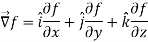
Is called gradient of f and we can write is as grad f.

So that-

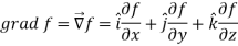
Here is a vector which has three components

Properties of gradient-

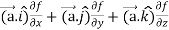
Property-1: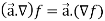

Proof:

First we will take left hand side

L.H.S =

=

=

=

Now taking R.H.S,

R.H.S. =

=

=

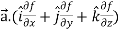
Here-                     L.H.S. = R.H.S.

Hence proved.

Property-2: Gradient of a constant (

Proof:

Suppose

Then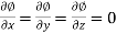

We know that the gradient-

= 0

Property-3: Gradient of the sum and difference of two functions-

If f and g are two scalar point functions, then

Proof:   

L.H.S                                

Hence proved

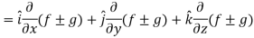
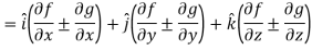
Property-4: Gradient of the product of two functions

If f and g are two scalar point functions, then

Proof:

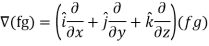
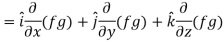
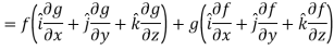
So that-

Hence proved.

Property-5: Gradient of the quotient of two functions-

If f and g are two scalar point functions, then-

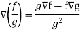
Proof:

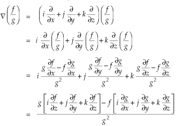
So that-

Example-1: If , then show that

1.

2.

Sol.

Suppose 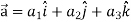  and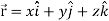

Now taking L.H.S,

Which is

Hence proved.

2.

So that

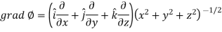
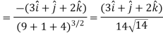
Example: If 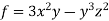then find grad f at the point (1,-2,-1).

Sol.

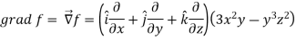
Now grad f at (1 , -2, -1) will be-       

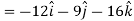
Example: If then prove that grad u , grad v and grad w are coplanar.

Sol.

Here-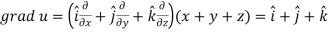                     

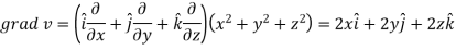
Now-

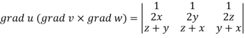
Apply

Which becomes zero.

So that we can say that grad u, grad v and grad w are coplanar vectors.

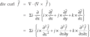
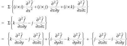
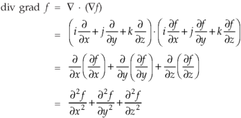
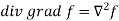
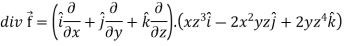
Divergence and Curl of a vector field

Divergence (Definition)-

Suppose is a given continuous differentiable vector function then the divergence of this function can be defined as-

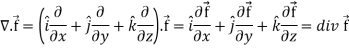
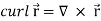
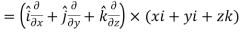
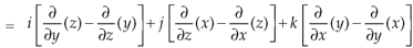
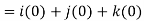
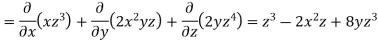
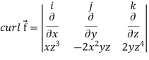
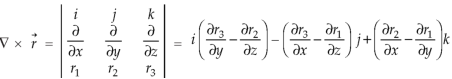
Curl (Definition)-

Curl of a vector function can be defined as-

Note- Irrotational vector-

If then the vector is said to be irrotational.

Vector identities:

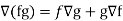
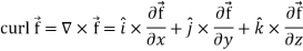
Identity-1:  grad uv = u grad v + v grad u

Proof: 

So that

Graduv = u grad v + v grad u

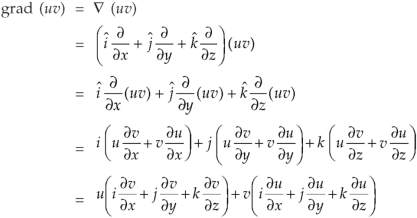
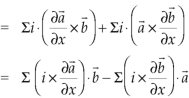
Identity-2: 

Proof:

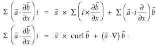
Interchanging , we get-

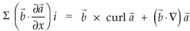
We get by using above equations-

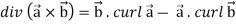
Identity-3

Proof: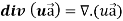   

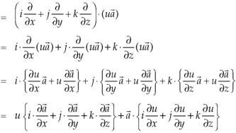
So that-

Identity-4

Proof:

So that,

Identity-5                  curl (u

Proof:

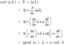
So that

Curl (u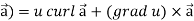

Identity-6:

Proof:

So that-

Identity-7: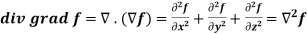

Proof:

So that-

Example-1: Show that-

1.

2.

Sol. We know that-

2. We know that-

= 0

Example-2: If then find the divergence and curl of .

Sol.  we know that-

Now-

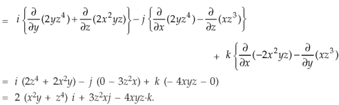
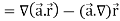
Example-3: Prove that

Note- here is a constant vector and

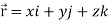
Sol. Here 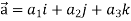   and

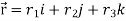
So that

Now-

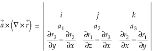
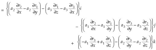
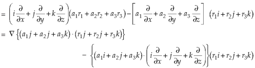
So that-

4.6. Directional derivative

Let ϕ be a scalar point function and let ϕ(P) and ϕ(Q) be the values of ϕ at two neighbouring points P and Q in the field. Then,

,are the directional derivative of ϕ in the direction of the coordinate axes at P.

The directional derivative of ϕ in the direction l, m, n=l + m+

The directional derivative of ϕ in the direction of =

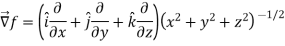
Example: Find the directional derivative of 1/r in the direction where

Sol. Here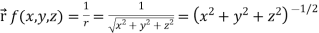

Now,

And

We know that-

So that-

Now

Directional derivative =

Example: Find the directional derivative of

At the points (3, 1, 2) in the direction of the vector .

Sol. Here it is given that-

Now at the point (3, 1, 2)-

Let be the unit vector in the given direction, then

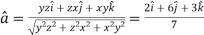at (3, 1, 2)

Now,

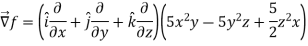
Example: Find the directional derivatives of at the point P(1, 1, 1) in the direction of the line

Sol. Here

Direction ratio of the line are 2, -2, 1

Now directions cosines of the line are-

Which are

Directional derivative in the direction of the line-

4.7. Line integrals, surface integrals, volume integrals

The Line Integral

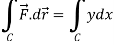
Let- F be vector function defined throughout some region of space and let C be any curve in that region. ṝis the position vector of a point p (x,y,z) on C then the integral ƪ F .dṝ is called the line integral of  F taken over

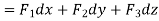
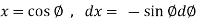
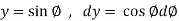
Now, since ṝ =xi+yi+zk

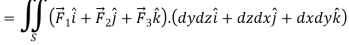
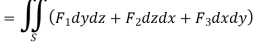
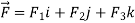
And if F͞ =F1i + F2 j+ F3  K

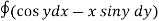
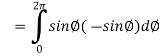
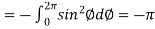
Q1. Evaluate where F= cos y.i-x siny j and C is the curve y= in the xy plae from (1,0) to (0,1)

Solution: The curve y= i.e x2+y2 =1. Is a circle with centre at the origin and radius unity.

=

=

=       =-1

Q2. Evaluate where = (2xy +z2) I +x2j +3xz2 k along the curve x=t, y=t2, z= t3 from (0,0,0) to (1,1,1).

Solution :  F x dr =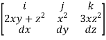

Put x=t, y=t2, z= t3

Dx=dt ,dy=2tdt,                dz=3t2dt.

F x dr =

=(3t4-6t8) dti  – ( 6t5+3t8 -3t7) dt j +( 4t4+2t7-t2)dt k

=t4-6t3)dti –(6t5+3t8-3t7)dt j+(4t4 + 2t7 – t2)dt k

=

=+

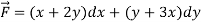
Example 3: Prove that   ͞͞͞F = [y2cos x +z3] i+(2y sin x – 4) j +(3xz2 + 2) k is a conservative field. Find (i) scalar potential for͞͞͞F  (ii) the work done in moving an object in this field from (0, 1, -1) to (/ 2,-1, 2)

Sol. : (a) The fleld is conservative if cur͞͞͞͞͞͞F = 0.

Now, curl͞͞͞F = ̷̷ X                    / y            / z

Y2COS X +Z3        2y sin x-4     3xz2 + 2

; Cur = (0-0) – (3z2 – 3z2) j + (2y cos x- 2y cos x) k = 0

; F is conservative.

(b) Since F is conservative there exists a scalar potential ȸ such that

F = ȸ

(y2cos x=z3) i + (2y sin x-4) j + (3xz2 + 2) k =   i +   j + k

= y2cos x + z3, = 2y sin x – 4, = 3xz2 + 2

Now, = dx + dy + dz

= (y2cos x + z3) dx +(2y sin x – 4)dy + (3xz2 + 2)dz

= (y2cos x dx + 2y sin x dy) +(z3dx +3xz2dz) +(- 4 dy) + (2 dz)

=d(y2 sin x + z3x – 4y -2z)

ȸ = y2 sin x +z3x – 4y -2z

(c)  now, work done = .d   ͞r

=  dx + (2y sin x – 4) dy + ( 3xz2 + 2) dz

=   (y2 sin x + z3x – 4y + 2z)    (as shown above)

= [ y2 sin x + z3x – 4y + 2z ]( /2, -1, 2)

= [ 1 +8 + 4 + 4 ] – { - 4 – 2} =4 + 15

Sums Based on Line Integral

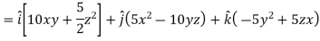
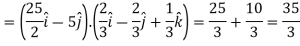
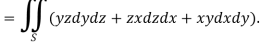
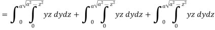
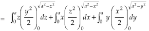
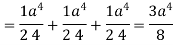
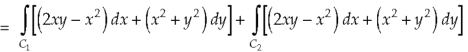
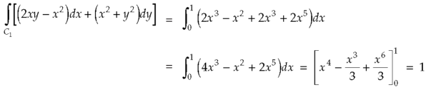
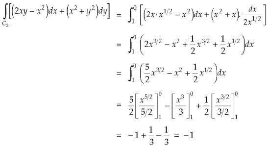
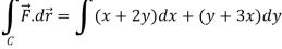
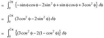
1. Evaluate where =yz i+zx  j+xy k and C is the position of the curve.

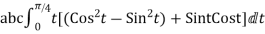
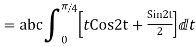
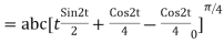
= (a cost)i+(b sint)j+ct k , from y=0 to t=π/4.

Soln.  = (a cost)i+(b sint)j+ct k

The parametric eqn. Of the curve are x= a cost, y=b sint, z=ct              (i)

=

Putting values of x,y,z from (i),

Dx=-a sint

Dy=b cost

Dz=c dt

=

=

==

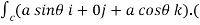
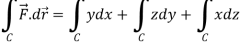
2. Find the circulation of around the curve C where =yi+zj+xk and C is circle .

Soln. Parametric eqn of circle are:

x=a cos

y=a sin

z=0

=xi+yj+zk = a cosi + b cos + 0 k

d=(-a sin i + a cos j)d

Circulation = =+zj+xk). d

=-a sin i + a cos j)d

= =

Surface integrals-

An integral which we evaluate over a surface is called a surface integral.

Surface integral =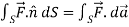

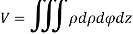
Volume integrals-

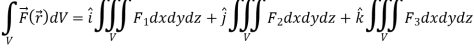
The volume integral is denoted by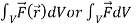

And defined as-

If  , then

Note-

If in a conservative field 

Then this is the condition for independence of path.

Example: Evaluate 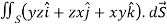, where S is the surface of the sphere in the first octant.

Sol. Here-

Which becomes-

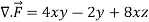
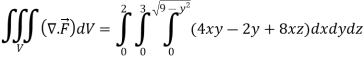
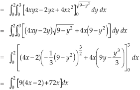
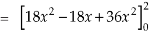
Example: Evaluate , where and V is the closed reason bounded by the planes 4x + 2y + z = 8, x = 0, y = 0, z = 0.

Sol.

Here-   4x + 2y + z = 8

Put y = 0 and z = 0 in this, we get

4x = 8 or x = 2

Limit of x varies from 0 to 2 and y varies from 0 to 4 – 2x

And z varies from 0 to 8 – 4x – 2y

So that-

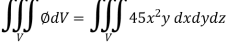
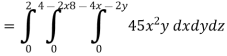
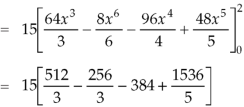
So that-

Example: Evaluate if V is the region in the first octant bounded by and the plane x = 2 and .

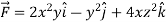Sol.

x varies from 0 to 2

The volume will be-

4.8. Green’s theorem, Stokes theorem and Gauss divergence theorem (Without proof)

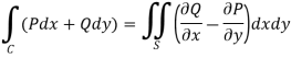
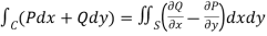
Green’s theorem in a plane

If C be a regular closed curve in the xy-plane and S is the region bounded by C then,

Where P and Q are the continuously differentiable functions inside and on C.

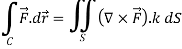
Green’s theorem in vector form-

Example-1: Apply Green’s theorem to evaluate where C is the boundary of the area enclosed by the x-axis and the upper half of circle

Sol. We know that by Green’s theorem-

And it it given that-

Now comparing the given integral-

P =   and   Q =

Now-

and

So that by Green’s theorem, we have the following integral-

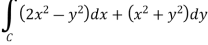
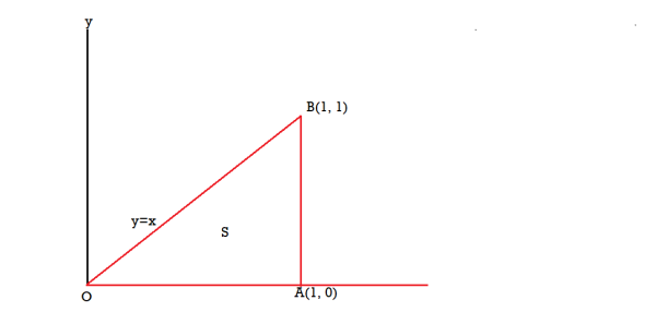
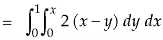
Example-2: Evaluate 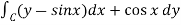by using Green’s theorem, where C is a triangle formed by

Sol. First we will draw the figure-

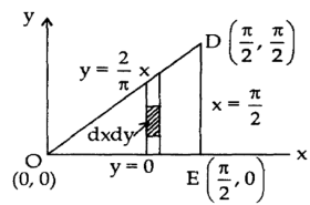
Here the vertices of triangle OED are (0,0), (

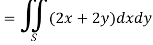
Now by using Green’s theorem-

Here P = y – sinx, and Q  =cosx

So that-

and

Now-

=

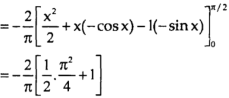
Which is the required answer.

Example-3: Verify green’s theorem in xy-plane for 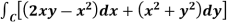where C is the boundary of the region enclosed by

Sol.

On comparing with green’s theorem,

We get-

P = and Q =

and

By using Green’s theorem-

  ………….. (1)

And left hand side=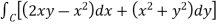

………….. (2)

Now,

Along

Along

Put these values in (2), we get-

L.H.S. = 1 – 1 = 0

So that the Green’s theorem is verified.

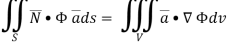
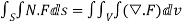
Gauss’s divergence theorem

Gauss divergence theorem

If V is the volume bounded by a closed surface S and is a vector point function with continuous derivative-

Then it can be written as-

Where unit vector to the surface S.

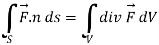
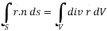
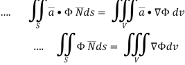
Example-1: Prove the following by using Gauss divergence theorem-

1.

2.

Where S is any closed surface having volume V and

Sol. Here we have by Gauss divergence theorem-

Where V is the volume enclose by the surface S.

We know that-

= 3V

2.

Because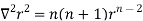 

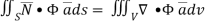
Example – 2 Show that 

Sol

By divergence theorem, 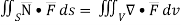 ..…(1)

Comparing  this  with  the  given  problem  let 

Hence, by (1)

                                    ………….(2)

Now ,

Hence, from (2), We get,

Example Based on Gauss Divergence Theorem

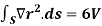
1. Show that

Soln.  We have Gauss Divergence Theorem

By data, F=  

=(n+3)

2 Prove that  =

Soln. By Gauss Divergence Theorem,

=

= =

.[

=

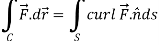
Stoke’s theorem (without proofs) and their verification

If is any continuously differentiable vector point function and S is a surface bounded by a curve C, then-

Example-1: Verify stoke’s theorem when and surface S is the part of sphere , above the xy-plane.

Sol.

We know that by stoke’s theorem,

Here C is the unit circle-

So that-

Now again on the unit circle C, z = 0

Dz = 0

Suppose, 

And           

Now

  ……………… (1)

Now-

Curl

Using spherical polar coordinates-

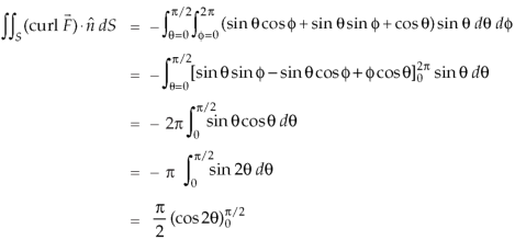
  ………………… (2)

From equation (1) and (2), stoke’s theorem is verified.

Example-2: If 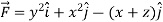and C is the boundary of the triangle with vertices at (0, 0, 0), (1, 0, 0) and (1, 1, 0), then evaluate by using Stoke’s theorem.

Sol. Here we see that z-coordinates of each vertex of the triangle is zero, so that the triangle lies in the xy-plane and

Now,

Curl

Curl

The equation of the line OB is y = x

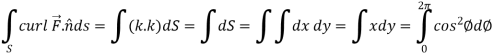
Now by stoke’s theorem,

Example-3: Verify Stoke’s theorem for the given function-

Where C is the unit circle in the xy-plane.

Sol. Suppose-

Here

We know that unit circle in xy-plane-

Or

So that,

Now

Curl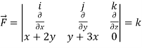

Now,

Hence the Stoke’s theorem is verified.