UNIT- 6

Recursion

6.1 Recursion

Recursion is the process which comes into existence when a function calls a copy of itself to work on a smaller problem. Any function which calls itself is called recursive function, and such function calls are called recursive calls. Recursion involves several numbers of recursive calls. However, it is important to impose a termination condition of recursion. Recursion code is shorter than iterative code however it is difficult to understand.

Recursion cannot be applied to all the problem, but it is more useful for the tasks that can be defined in terms of similar subtasks. For Example, recursion may be applied to sorting, searching, and traversal problems.

Generally, iterative solutions are more efficient than recursion since function call is always overhead. Any problem that can be solved recursively, can also be solved iteratively. However, some problems are best suited to be solved by the recursion, for example, tower of Hanoi, Fibonacci series, factorial finding, etc.

In the following example, recursion is used to calculate the factorial of a number.

1. #include <stdio.h>  
2. Int fact (int);  
3. Int main()  
4. {  
5.    Int n,f;  
6.    Printf("Enter the number whose factorial you want to calculate?");  
7.    Scanf("%d",&n);  
8.    f = fact(n);  
9.    Printf("factorial = %d",f);  
10. }  
11. Int fact(int n)  
12. {  
13.    If (n==0)  
14.    {  
15.        Return 0;  
16.    }  
17.    Else if ( n == 1)  
18.    {  
19.        Return 1;  
20.    }  
21.    Else   
22.    {  
23.        Return n*fact(n-1);  
24.    }  
25. }  

Output

Enter the number whose factorial you want to calculate?5

Factorial = 120

We can understand the above program of the recursive method call by the figure given below:

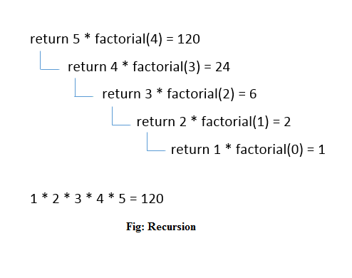
Recursive Function

A recursive function performs the tasks by dividing it into the subtasks. There is a termination condition defined in the function which is satisfied by some specific subtask. After this, the recursion stops and the final result is returned from the function.

The case at which the function doesn't recur is called the base case whereas the instances where the function keeps calling itself to perform a subtask, is called the recursive case. All the recursive functions can be written using this format.

Pseudocode for writing any recursive function is given below.

1. If (test_for_base)  
2. {  
3.    Return some_value;  
4. }  
5. Else if (test_for_another_base)  
6. {  
7.    Return some_another_value;  
8. }  
9. Else  
10. {  
11.    // Statements;  
12.    Recursive call;  
13. }  

Example of recursion in C

Let's see an example to find the nth term of the Fibonacci series.

1. #include<stdio.h>  
2. Int fibonacci(int);  
3. Void main ()  
4. {  
5.    Int n,f;  
6.    Printf("Enter the value of n?");  
7.    Scanf("%d",&n);  
8.    f = fibonacci(n);  
9.    Printf("%d",f);  
10. }  
11. Int fibonacci (int n)  
12. {  
13.    If (n==0)  
14.    {  
15.    Return 0;  
16.    }  
17.    Else if (n == 1)  
18.    {  
19.        Return 1;   
20.    }  
21.    Else  
22.    {  
23.        Return fibonacci(n-1)+fibonacci(n-2);  
24.    }  
25. }  

Output

Enter the value of n?12

144

Memory allocation of Recursive method

Each recursive call creates a new copy of that method in the memory. Once some data is returned by the method, the copy is removed from the memory. Since all the variables and other stuff declared inside function get stored in the stack, therefore a separate stack is maintained at each recursive call. Once the value is returned from the corresponding function, the stack gets destroyed. Recursion involves so much complexity in resolving and tracking the values at each recursive call. Therefore we need to maintain the stack and track the values of the variables defined in the stack.

Let us consider the following example to understand the memory allocation of the recursive functions.

1. Int display (int n)  
2. {  
3.    If(n == 0)  
4.        Return 0; // terminating condition  
5.    Else   
6.    {  
7.        Printf("%d",n);  
8.        Return display(n-1); // recursive call  
9.    }  
10. }  

Explanation

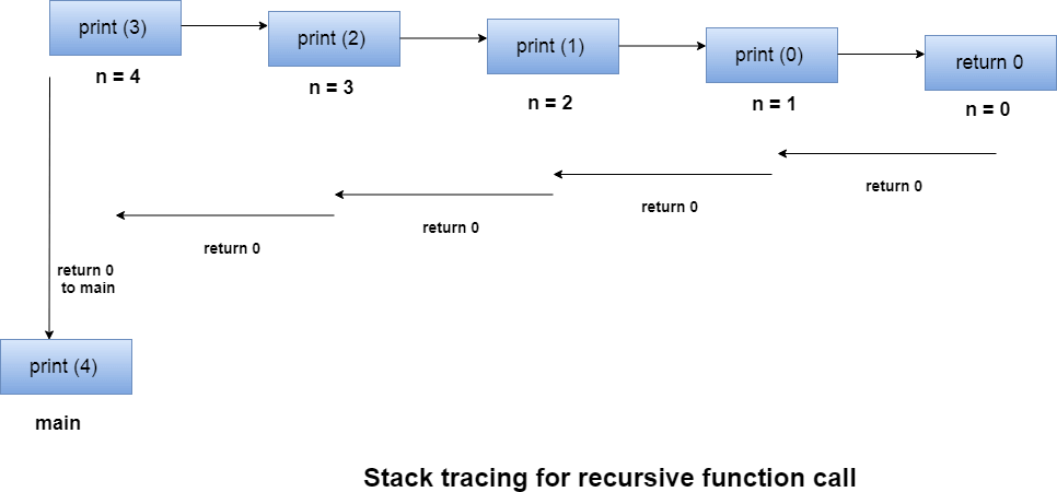
Let us examine this recursive function for n = 4. First, all the stacks are maintained which prints the corresponding value of n until n becomes 0, Once the termination condition is reached, the stacks get destroyed one by one by returning 0 to its calling stack. Consider the following image for more information regarding the stack trace for the recursive functions.

6.2 Recursion as a different way of solving problems

Recursion is a common form of the general-purpose problem-solving technique called divide and conquer''. The principle of divide-and-conquer, is that you solve a given problem P in 3 steps:

1. Divide P into several subproblems, P1,P2,...Pn.
2. Solve, however you can, each of the subproblems to get solutions S1...Sn.
3. Use S1...Sn to construct a solution to the original problem, P.

This is often recursive, because in order to solve one or more of the subproblems, you might use this very same strategy. For instance, you might solve P1 be subdividing it into P1a,P1b..., solving each one of them, and putting together their solutions to get the solution S1 to problem P1.

An Everyday Example

To give a simple example, suppose you want to solve this problem:

P = carry a pile of 50 books from your office to your car.

Well, you can't even lift such a big pile, never mind carry it. So you split the original pile into 3 piles:

P1 contains 10 books, P2 contains 15 books, P3 contains 25 books.

Your plan, of course, is to carry each pile to the car separately, and then put them back together into one big pile once they are all there. This is a recursive divide-and-conquer strategy; you have divided the original problem P into 3 problems of the same kind.

Now suppose you can directly solve P1 and P2 - they are small enough that you can carry them to the car. So, P1 and P2 are now sitting out there by the car. Once you get P3 there, you will pile them up again.

But P3 is too big to be carried. You apply the same strategy recursively: divide P3 into smaller problems, solve them, and combine the results to make the solution for P3. You divide P3 into two piles, P3a has 11 books, P3b has 14, and carry these separately to the car. Then you put P3a back onto P3b to form the pile P3 there at the car.

Now you have solved all the subproblems: P1, P2, P3 are sitting at the car. You stack them into one big pile, and presto, you have solved the original problem.

This may seem like a rather hokey example, but it illustrates very well the principles of divide-and-conquer. Let us see how we can use the very same ideas to solve mathematical and computer science problems.

A Mathematical Example

Find an algorithm for raising a number X to the power N, where N is a positive integer. You may use only two operations: multiplication, subtraction. We would like to multiply N copies of X all at once, but, like the piles of books, we do not have an operation that directly allows us to do that: we can only multiply two numbers at a time. In other words, the problems we can solve directly are these:

• Raise X to the power 1: answer = X.
• Raise X to the power 2: answer = X * X.

Any other problem we have to solve indirectly, by breaking it down into smaller and smaller problems until we have reduced it to one of these base cases.

So, if N > 2, we split the original problem into two subproblems:

• P1: raise X to the power I. The answer to this is S1.
• P2: raise X to the power N-I. The answer to this is S2.
• To get the final answer, S, combine S1 and S2: S = S1 * S2.

How do we solve P1 and P2? They are problems of exactly the same type as original problem, so we can apply to them exactly the same strategy that we applied to the original problem. We check to see if we can solve them directly... If I=1 or I=2 we can solve P1 directly; if N-I=1 or N-I=2 we can solve P2 directly. The problems we cannot solve directly, we solve recursively, as just described. An interesting feature of this strategy is that it works no matter how we split up N.

We can't directly solve this problem, so we divide it into:

• P1: raise 3 to the power 2. (choose I=2, no particular reason)
• P2: raise 3 to the power 5.

We can directly solve P1, the answer is S1 = 9. But P2 we have to further decompose:

• P2.1: raise 3 to the power 1. (choose I=1, no particular reason)
• P2.2: raise 3 to the power 4.

Again, P2.1 can be directly solved, S2.1 = 3, but P2.2 must be further decomposed:

• P2.2.1: raise 3 to the power 2.
• P2.2.2: raise 3 to the power 2.

These both can be directly solved; S2.2.1 = S2.2.2 = 9. These are combined to give S2.2 = 9*9 = 81.

Now that we have the solutions to P2.1 and P2.2 we combine them to get the solution to P2, S2 = 3*81 = 243.

Now that we have solutions for P1 and P2, we combine them to get the final solution, S = S1*S2 = 9*243 = 2187.

I said that the strategy would work no matter how we chose to subdivide the problem: any choice of I' will give the correct answer. However, some choices of I' compute the final answer faster than others. Which do you think is faster: choosing I=1 (every time) or I=2?

Answer:The computation will be faster if you choose I=2 because there will be half the number of recursive calls, and therefore half the overhead.

This is true of most recursive strategies: they usually work correctly for many different ways of decomposing the problem, but some ways are much more efficient than others. In our first example, we also were free to divide the pile of books into as many piles and whatever sizes we liked. But it obviously would be very inefficient to carry one book at a time.

Data Structures Examples

Many problems involving data structures are naturally solved recursively. This is because most data structures are collections of components and they can easily be divided into subcollections that can be independently processed, just as, in our first example, we divided the pile of books into smaller piles that could be carried to the car separately.

For example, suppose we want to add up the numbers stored in array X between positions FIRST and LAST. We can solve this directly in two very simple cases:

FIRST=LAST:

There is one number to be added, the answer is X[FIRST].

FIRST+1=LAST:

There are 2 numbers to be added, the answer is X[FIRST] + X[LAST].

Otherwise, there are too many numbers to be added all at once, so we divide the problem into two subproblems by dividing the array into two parts:

• P1: add up the numbers in X between positions FIRST and M; the answer is S1.
• P2: add up the numbers in X between positions M+1 and LAST; the answer is S2.

The final answer is obtained by combining S1 and S2 in an appropriate way. In order to get the sum of all the numbers in the array, we add together the two partial sums: S = S1 + S2.

The exact way we divide up the array does not affect the correctness of this strategy: M can be any value at all, FIRST<M<LAST.

The structure' of the collection dictates which are the easiest ways to divide up the collection. As we've just seen arrays are very flexible, it is easy to divide them into a front and a back at any division point we care to choose. Other data structures are easily divided only in certain ways.

For example, suppose we want to add up all the numbers in a stack. We'll base our solution on the recursive definition of stack we saw earlier: a stack is Empty, or has 2 parts, Top and Remainder.

We can directly add up all the numbers in an Empty stack! There are none, and by convention, the sum of no numbers is 0.

To add up the numbers in a non-empty stack, we will divide the stack into two parts, add up the parts separately, and combine the results. This is exactly what we did for arrays, but now we have to think, what is an easy way to divide a stack into two parts?

The definition of stack gives us an immediate answer: a stack naturally decomposes into a Top element (which is a number, not a stack), and a Remainder, which is a stack. So we can decompose the problem of adding up the numbers in a nonempty stack into these two subproblems:

• P1: add up all the numbers in the Top part. This is not a recursive call, because Top is not a stack. In fact, Top is just a number, so the solution to this subproblem is just the top value itself. S1=Top value.
• P2: add up all the numbers in Remainder. This is a recursive call, because Remainder is a stack. The solution is S2.

Now, combine S1 and S2 in the appropriate way to construct the final solution: S=S1+S2, or, S=Top value + S2.

Of course, there is nothing special about adding'. The very same strategy would work if we wanted to multiply together all the values in a collection, to find the largest value, to print out the elements, to count the number of elements, and so on.

Suppose we wished to sort the values in array X between positions FIRST and LAST. We can solve this directly in two very simple cases:

FIRST=LAST:

There is one number to be sorted, nothing needs to be done.

FIRST+1=LAST:

There are 2 numbers to be sorted; compare them and, if they are out of order, swap them.

Otherwise, there are too many numbers to be sorted all at once, so we divide the problem into two subproblems by dividing the array into two parts:

• P1: sort the numbers in X between positions FIRST and M; the answer is S1.
• P2: sort the numbers in X between positions M+1 and LAST; the answer is S2.

The final answer is obtained by combining S1 and S2 in an appropriate way. The method for combining them is called merging', and it is a simple, efficient process. You can read about it in the textbook (section 5.4) or wait until we study sorting in detail later in the course.

As before, the exact way we divide up the array does not affect the correctness of this strategy: M can be any value at all, FIRST<M<LAST. Certain values of M correspond to well-known sorting algorithms:

M = 1

Gives rise to the sorting algorithm called insertion sort.

M = the midpoint between FIRST and LAST

Gives rise to the MergeSort algorithm.

Both are correct, but their efficiency is very different: MergeSort is extremely fast (optimal in fact), whereas insertion sort is very slow.

6.3 Example programs such as Finding Factorial, Fibonacci series, Ackerman function etc.

Factorial Program in C

Factorial Program in C: Factorial of n is the product of all positive descending integers. Factorial of n is denoted by n!. For example:

1. 5! = 5*4*3*2*1 = 120  
2. 3! = 3*2*1 = 6  

Here, 5! is pronounced as "5 factorial", it is also called "5 bang" or "5 shriek".

The factorial is normally used in Combinations and Permutations (mathematics).

There are many ways to write the factorial program in c language. Let's see the 2 ways to write the factorial program.

• Factorial Program using loop
• Factorial Program using recursion

Factorial Program using loop

Let's see the factorial Program using loop.

1. #include<stdio.h>  
2. Int main()    
3. {    
4. Int i,fact=1,number;    
5. Printf("Enter a number: ");    
6.  Scanf("%d",&number);    
7.    For(i=1;i<=number;i++){    
8.      Fact=fact*i;    
9.  }    
10.  Printf("Factorial of %d is: %d",number,fact);    
11. Return 0;  
12. }   

Output:

Enter a number: 5

Factorial of 5 is: 120

Factorial Program using recursion in C

Let's see the factorial program in c using recursion.

1. #include<stdio.h>  
2.  
3. Long factorial(int n)  
4. {  
5.  If (n == 0)  
6.    Return 1;  
7.  Else  
8.    Return(n * factorial(n-1));  
9. }  
10.   
11. Void main()  
12. {  
13.  Int number;  
14.  Long fact;  
15.  Printf("Enter a number: ");  
16.  Scanf("%d", &number);   
17.   
18.  Fact = factorial(number);  
19.  Printf("Factorial of %d is %ld\n", number, fact);  
20.  Return 0;  
21. }  

Output:

Enter a number: 6

Factorial of 5 is: 720

Fibonacci Series in C

In case of fibonacci series, next number is the sum of previous two numbers for example 0, 1, 1, 2, 3, 5, 8, 13, 21 etc. The first two numbers of fibonacci series are 0 and 1.

There are two ways to write the fibonacci series program:

• Fibonacci Series without recursion
• Fibonacci Series using recursion

Fibonacci Series in C without recursion

Let's see the fibonacci series program in c without recursion.

1. #include<stdio.h>    
2. Int main()    
3. {    
4. Int n1=0,n2=1,n3,i,number;    
5. Printf("Enter the number of elements:");    
6. Scanf("%d",&number);    
7. Printf("\n%d %d",n1,n2);//printing 0 and 1    
8. For(i=2;i<number;++i)//loop starts from 2 because 0 and 1 are already printed    
9. {    
10.  n3=n1+n2;    
11.  Printf(" %d",n3);    
12.  n1=n2;    
13.  n2=n3;    
14. }  
15.  Return 0;  
16. }    

Output:

Enter the number of elements:15

0 1 1 2 3 5 8 13 21 34 55 89 144 233 377

Fibonacci Series using recursion in C

Let's see the fibonacci series program in c using recursion.

1. #include<stdio.h>    
2. Void printFibonacci(int n){    
3.    Static int n1=0,n2=1,n3;    
4.    If(n>0){    
5.         n3 = n1 + n2;    
6.         n1 = n2;    
7.         n2 = n3;    
8.         Printf("%d ",n3);    
9.         PrintFibonacci(n-1);    
10.    }    
11. }    
12. Int main(){    
13.    Int n;    
14.    Printf("Enter the number of elements: ");    
15.    Scanf("%d",&n);    
16.    Printf("Fibonacci Series: ");    
17.    Printf("%d %d ",0,1);    
18.    PrintFibonacci(n-2);//n-2 because 2 numbers are already printed    
19.  Return 0;  
20. }    

Output:

Enter the number of elements:15

0 1 1 2 3 5 8 13 21 34 55 89 144 233 377

Ackerman function

In computability theory, the Ackermann function, named after Wilhelm Ackermann, is one of the simplest and earliest-discovered examples of a total computable function that is not primitive recursive. All primitive recursive functions are total and computable, but the Ackermann function illustrates that not all total computable functions are primitive recursive.

It’s a function with two arguments each of which can be assigned any non-negative integer.

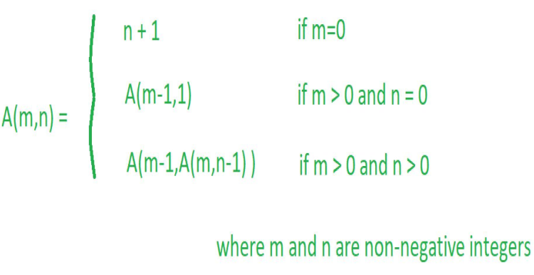
Ackermann function is defined as:

Ackermann algorithm:

Ackermann(m, n)

{next and goal are arrays indexed from 0 to m, initialized so that next[O]

Through next[m] are 0, goal[O] through goal[m - l] are 1, and goal[m] is -1}

Repeat

Value<-- next[O] + 1

Transferring<-- true

Current<-- O

While transferring do begin

If next[current] = goal[current] then goal[current] <-- value

Else transferring <-- false

Next[current] <-- next[current]+l

Current<-- current + 1

End while

Until next[m] = n + 1

Return value {the value of A(m, n)}

End Ackermann

Here’s the explanation of the given Algorithm:
Let me explain the algorithm by taking the example A(1, 2) where m = 1 and n = 2
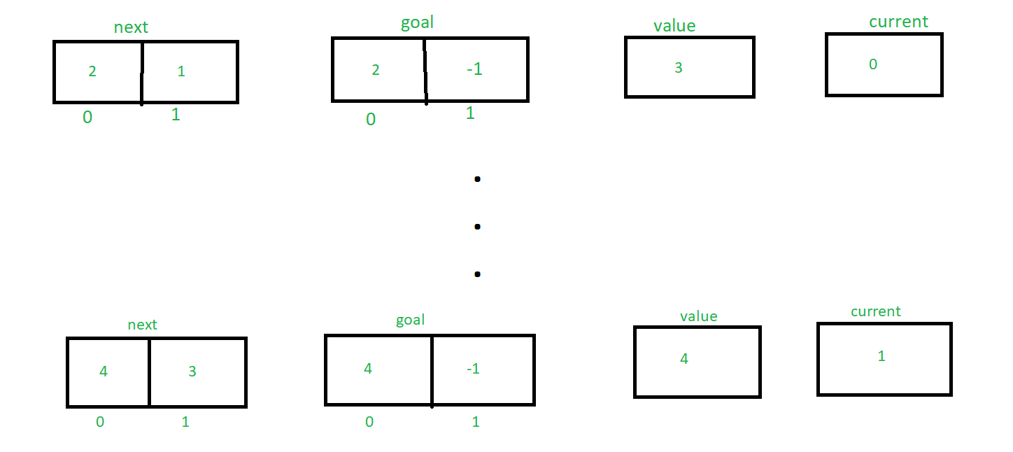
So according to the algorithm initially the value of next, goal, value and current are:

Though next[current] != goal[current], so else statement will execute and transferring become false.
So now, the value of next, goal, value and current are:

Similarly by tracing the algorithm until next[m] = 3 the value of next, goal, value and current are changing accordingly. Here’s the explanation how the values are changing,

Finally returning the valuee.g 4

Analysis of this algorithm:

• The time complexity of this algorithm is: O(mA(m, n)) to compute A(m, n)
• The space complexity of this algorithm is: O(m) to compute A(m, n)

Let’s understand the definition by solving a problem!

Solve A(1, 2)?

Answer:

Given problem is A(1, 2)
Here m = 1, n = 2 e.g m > 0 and n > 0
Hence applying third condition of Ackermann function
A(1, 2) = A(0, A(1, 1)) ———- (1)
Now, Let’s find A(1, 1) by applying third condition of Ackermann function
A(1, 1) = A(0, A(1, 0)) ———- (2)
Now, Let’s find A(1, 0) by applying second condition of Ackermann function
A(1, 0) = A(0, 1) ———- (3)
Now, Let’s find A(0, 1) by applying first condition of Ackermann function
A(0, 1) = 1 + 1 = 2
Now put this value in equation 3
Hence A(1, 0) = 2
Now put this value in equation 2
A(1, 1) = A(0, 2) ———- (4)
Now, Let’s find A(0, 2) by applying first condition of Ackermann function
A(0, 2) = 2 + 1 = 3
Now put this value in equation 4
Hence A(1, 1) = 3
Now put this value in equation 1
A(1, 2) = A(0, 3) ———- (5)
Now, Let’s find A(0, 3) by applying first condition of Ackermann function
A(0, 3) = 3 + 1 = 4
Now put this value in equation 5
Hence A(1, 2) = 4

So, A (1, 2) = 4

Let’s solve another two questions on this by yourself!

Question: Solve A(2, 1)?
Answer: 5

Question: Solve A(2, 2)?
Answer: 7

Here is the simplest c and python recursion function code for generating Ackermann function

6.4 Quick sort or Merge sort

Quick Sort

Quick sort is a highly efficient sorting algorithm and is based on partitioning of array of data into smaller arrays. A large array is partitioned into two arrays one of which holds values smaller than the specified value, say pivot, based on which the partition is made and another array holds values greater than the pivot value.

Quicksort partitions an array and then calls itself recursively twice to sort the two resulting subarrays. This algorithm is quite efficient for large-sized data sets as its average and worst-case complexity are O(nLogn) and image.png(n2), respectively.

Partition in Quick Sort

Following animated representation explains how to find the pivot value in an array.

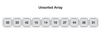
The pivot value divides the list into two parts. And recursively, we find the pivot for each sub-lists until all lists contains only one element.

Quick Sort Pivot Algorithm

Based on our understanding of partitioning in quick sort, we will now try to write an algorithm for it, which is as follows.

Step 1− Choose the highest index value has pivot

Step 2− Take two variables to point left and right of the list excluding pivot

Step 3− left points to the low index

Step 4− right points to the high

Step 5− while value at left is less than pivot move right

Step 6− while value at right is greater than pivot move left

Step 7− if both step 5 and step 6 does not match swap left and right

Step 8− if left ≥ right, the point where they met is new pivot

Quick Sort Pivot Pseudocode

The pseudocode for the above algorithm can be derived as −

FunctionpartitionFunc(left, right, pivot)

LeftPointer= left

RightPointer= right -1

WhileTruedo

While A[++leftPointer]< pivot do

//do-nothing           

Endwhile

WhilerightPointer>0&& A[--rightPointer]> pivot do

//do-nothing        

Endwhile

IfleftPointer>=rightPointer

Break

Else

SwapleftPointer,rightPointer

Endif

Endwhile

SwapleftPointer,right

ReturnleftPointer

Endfunction

Quick Sort Algorithm

Using pivot algorithm recursively, we end up with smaller possible partitions. Each partition is then processed for quick sort. We define recursive algorithm for quicksort as follows −

Step 1− Make the right-most index value pivot

Step 2− partition the array using pivot value

Step 3− quicksort left partition recursively

Step 4− quicksort right partition recursively

Quick Sort Pseudocode

To get more into it, let see the pseudocode for quick sort algorithm −

ProcedurequickSort(left, right)

If right-left <=0

Return

Else

Pivot= A[right]

Partition=partitionFunc(left, right, pivot)

QuickSort(left,partition-1)

QuickSort(partition+1,right)

Endif  

End procedure

Quick Sort Program in C

Quick sort is a highly efficient sorting algorithm and is based on partitioning of array of data into smaller arrays. A large array is partitioned into two arrays one of which holds values smaller than the specified value, say pivot, based on which the partition is made and another array holds values greater than the pivot value.

Implementation in C

#include<stdio.h>

#include<stdbool.h>

#define MAX 7

IntintArray[MAX]={4,6,3,2,1,9,7};

Voidprintline(int count){

Inti;

For(i=0;i < count-1;i++){

Printf("=");

}

Printf("=\n");

}

Void display(){

Inti;

Printf("[");

// navigate through all items

For(i=0;i <MAX;i++){

Printf("%d ",intArray[i]);

}

Printf("]\n");

}

Void swap(int num1,int num2){

Int temp =intArray[num1];

IntArray[num1]=intArray[num2];

IntArray[num2]= temp;

}

Int partition(int left,int right,int pivot){

IntleftPointer= left -1;

IntrightPointer= right;

While(true){

While(intArray[++leftPointer]< pivot){

//do nothing

}

While(rightPointer>0&&intArray[--rightPointer]> pivot){

//do nothing

}

If(leftPointer>=rightPointer){

Break;

}else{

Printf(" item swapped :%d,%d\n",intArray[leftPointer],intArray[rightPointer]);

Swap(leftPointer,rightPointer);

}

}

Printf(" pivot swapped :%d,%d\n",intArray[leftPointer],intArray[right]);

Swap(leftPointer,right);

Printf("Updated Array: ");

Display();

ReturnleftPointer;

}

VoidquickSort(int left,int right){

If(right-left <=0){

Return;

}else{

Int pivot =intArray[right];

IntpartitionPoint= partition(left, right, pivot);

QuickSort(left,partitionPoint-1);

QuickSort(partitionPoint+1,right);

}

}

Int main(){

Printf("Input Array: ");

Display();

Printline(50);

QuickSort(0,MAX-1);

Printf("Output Array: ");

Display();

Printline(50);

}

If we compile and run the above program, it will produce the following result −

Output

Input Array: [4 6 3 2 1 9 7 ]

==================================================

Pivot swapped :9,7

Updated Array: [4 6 3 2 1 7 9 ]

Pivot swapped :4,1

Updated Array: [1 6 3 2 4 7 9 ]

Item swapped :6,2

Pivot swapped :6,4

Updated Array: [1 2 3 4 6 7 9 ]

Pivot swapped :3,3

Updated Array: [1 2 3 4 6 7 9 ]

Output Array: [1 2 3 4 6 7 9 ]

==================================================

Merge sort

Merge sort is the algorithm which follows divide and conquer approach. Consider an array A of n number of elements. The algorithm processes the elements in 3 steps.

1. If A Contains 0 or 1 elements then it is already sorted, otherwise, Divide A into two sub-array of equal number of elements.
2. Conquer means sort the two sub-arrays recursively using the merge sort.
3. Combine the sub-arrays to form a single final sorted array maintaining the ordering of the array.

The main idea behind merge sort is that, the short list takes less time to be sorted.

Complexity

Example :

Consider the following array of 7 elements. Sort the array by using merge sort.

1. A = {10, 5, 2, 23, 45, 21, 7}  

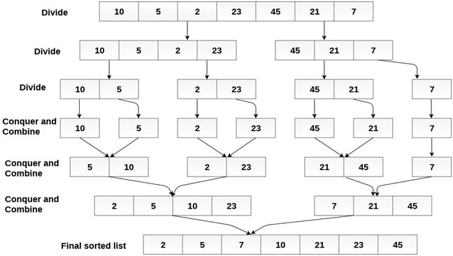
Algorithm

• Step 1: [INITIALIZE] SET I = BEG, J = MID + 1, INDEX = 0
• Step 2: Repeat while (I <= MID) AND (J<=END)
  IF ARR[I] < ARR[J]
  SET TEMP[INDEX] = ARR[I]
  SET I = I + 1
  ELSE
  SET TEMP[INDEX] = ARR[J]
  SET J = J + 1
  [END OF IF]
  SET INDEX = INDEX + 1
  [END OF LOOP]
  Step 3: [Copy the remaining
  elements of right sub-array, if
  any]
  IF I > MID
  Repeat while J <= END
  SET TEMP[INDEX] = ARR[J]
  SET INDEX = INDEX + 1, SET J = J + 1
  [END OF LOOP]
  [Copy the remaining elements of
  left sub-array, if any]
  ELSE
  Repeat while I <= MID
  SET TEMP[INDEX] = ARR[I]
  SET INDEX = INDEX + 1, SET I = I + 1
  [END OF LOOP]
  [END OF IF]
• Step 4: [Copy the contents of TEMP back to ARR] SET K = 0
• Step 5: Repeat while K < INDEX
  SET ARR[K] = TEMP[K]
  SET K = K + 1
  [END OF LOOP]
• Step 6: Exit

MERGE_SORT(ARR, BEG, END)

• Step 1: IF BEG < END
  SET MID = (BEG + END)/2
  CALL MERGE_SORT (ARR, BEG, MID)
  CALL MERGE_SORT (ARR, MID + 1, END)
  MERGE (ARR, BEG, MID, END)
  [END OF IF]
• Step 2: END

C Program

1. #include<stdio.h>  
2. Void mergeSort(int[],int,int);  
3. Void merge(int[],int,int,int);  
4. Void main ()  
5. {  
6.    Int a[10]= {10, 9, 7, 101, 23, 44, 12, 78, 34, 23};  
7.    Int i;  
8.    MergeSort(a,0,9);  
9.    Printf("printing the sorted elements");  
10.    For(i=0;i<10;i++)  
11.    {  
12.        Printf("\n%d\n",a[i]);  
13.    }  
14.      
15. }  
16. Void mergeSort(int a[], int beg, int end)  
17. {  
18.    Int mid;  
19.    If(beg<end)  
20.    {  
21.        Mid = (beg+end)/2;  
22.        MergeSort(a,beg,mid);  
23.        MergeSort(a,mid+1,end);  
24.        Merge(a,beg,mid,end);  
25.    }  
26. }  
27. Void merge(int a[], int beg, int mid, int end)  
28. {  
29.    Int i=beg,j=mid+1,k,index = beg;  
30.    Int temp[10];  
31.    While(i<=mid && j<=end)  
32.    {  
33.        If(a[i]<a[j])  
34.        {  
35.            Temp[index] = a[i];  
36.            i = i+1;  
37.        }  
38.        Else   
39.        {  
40.            Temp[index] = a[j];  
41.            j = j+1;   
42.        }  
43.        Index++;  
44.    }  
45.    If(i>mid)  
46.    {  
47.        While(j<=end)  
48.        {  
49.            Temp[index] = a[j];  
50.            Index++;  
51.            j++;  
52.        }  
53.    }  
54.    Else   
55.    {  
56.        While(i<=mid)  
57.        {  
58.            Temp[index] = a[i];  
59.            Index++;  
60.            i++;  
61.        }  
62.    }  
63.    k = beg;  
64.    While(k<index)  
65.    {  
66.        a[k]=temp[k];  
67.        k++;  
68.    }  
69. }  

Output:

Printing the sorted elements

7

9

10

12

23

23

34

44

78

101

Java Program

1. Public class MyMergeSort  
2. {  
3. Void merge(int arr[], int beg, int mid, int end)  
4. {  
5.  
6. Int l = mid - beg + 1;  
7. Int r = end - mid;  
8.  
9. IntLeftArray[] = new int [l];  
10. IntRightArray[] = new int [r];  
11.  
12. For (int i=0; i<l; ++i)  
13. LeftArray[i] = arr[beg + i];  
14.  
15. For (int j=0; j<r; ++j)  
16. RightArray[j] = arr[mid + 1+ j];  
17.  
18.  
19. Int i = 0, j = 0;  
20. Int k = beg;  
21. While (i<l&&j<r)  
22. {  
23. If (LeftArray[i] <= RightArray[j])  
24. {  
25. Arr[k] = LeftArray[i];  
26. i++;  
27. }  
28. Else  
29. {  
30. Arr[k] = RightArray[j];  
31. j++;  
32. }  
33. k++;  
34. }  
35. While (i<l)  
36. {  
37. Arr[k] = LeftArray[i];  
38. i++;  
39. k++;  
40. }  
41.  
42. While (j<r)  
43. {  
44. Arr[k] = RightArray[j];  
45. j++;  
46. k++;  
47. }  
48. }  
49.  
50. Void sort(int arr[], int beg, int end)  
51. {  
52. If (beg<end)  
53. {  
54. Int mid = (beg+end)/2;  
55. Sort(arr, beg, mid);  
56. Sort(arr , mid+1, end);  
57. Merge(arr, beg, mid, end);  
58. }  
59. }  
60. Public static void main(String args[])  
61. {  
62. Intarr[] = {90,23,101,45,65,23,67,89,34,23};  
63. MyMergeSort ob = new MyMergeSort();  
64. Ob.sort(arr, 0, arr.length-1);  
65.  
66. System.out.println("\nSorted array");  
67. For(int i =0; i<arr.length;i++)  
68. {  
69.    System.out.println(arr[i]+"");  
70. }  
71. }  
72. }  

Output:

Sorted array

23

23

23

34

45

65

67

89

90

101

C# Program

1. Using System;  
2. Public class MyMergeSort  
3. {  
4. Void merge(int[] arr, int beg, int mid, int end)  
5. {  
6.  
7. Int l = mid - beg + 1;  
8. Int r = end - mid;  
9.        Int i,j;  
10.  
11. Int[] LeftArray = new int [l];  
12. Int[] RightArray = new int [r];  
13.  
14. For (i=0; i<l; ++i)  
15. LeftArray[i] = arr[beg + i];  
16.  
17. For (j=0; j<r; ++j)  
18. RightArray[j] = arr[mid + 1+ j];  
19.  
20.  
21. i = 0; j = 0;  
22. Int k = beg;  
23. While (i < l && j < r)  
24. {  
25. If (LeftArray[i] <= RightArray[j])  
26. {  
27. Arr[k] = LeftArray[i];  
28. i++;  
29. }  
30. Else  
31. {  
32. Arr[k] = RightArray[j];  
33. j++;  
34. }  
35. k++;  
36. }  
37. While (i < l)  
38. {  
39. Arr[k] = LeftArray[i];  
40. i++;  
41. k++;  
42. }  
43.  
44. While (j < r)  
45. {  
46. Arr[k] = RightArray[j];  
47. j++;  
48. k++;  
49. }  
50. }  
51.  
52. Void sort(int[] arr, int beg, int end)  
53. {  
54. If (beg < end)  
55. {  
56. Int mid = (beg+end)/2;  
57. Sort(arr, beg, mid);  
58. Sort(arr , mid+1, end);  
59. Merge(arr, beg, mid, end);  
60. }  
61. }  
62. Public static void Main()  
63. {  
64. Int[] arr = {90,23,101,45,65,23,67,89,34,23};  
65. MyMergeSort ob = new MyMergeSort();  
66. Ob.sort(arr, 0, 9);  
67.  
68. Console.WriteLine("\nSorted array");  
69. For(int i =0; i<10;i++)  
70. {  
71.    Console.WriteLine(arr[i]+"");  
72. }  
73. }  
74. }  

Output:

Sorted array

23

23

23

34

45

65

67

89

90

101

Text Books

(i) Byron Gottfried, Schaum's Outline of Programming with C, McGraw-Hill

(ii) E. Balaguruswamy, Programming in ANSI C, Tata McGraw-Hill

Reference Books

(i) Brian W. Kernighan and Dennis M. Ritchie, The C Programming Language, Prentice Hall of India.