Unit–3
Basic Statistics
Professor Bowley defines the average as-
“Statistical constants which enable us to comprehend in a single effort the significance of the whole”
An average is a single value which is the best representative for a given data set.
Measures of central tendency show the tendency of some central values around which data tend to cluster.
The following are the various measures of central tendency-
1. Arithmetic mean
2. Median
3. Mode
4. Weighted mean
5. Geometric mean
6. Harmonic mean
Arithmetic mean or mean-
Arithmetic mean is a value which is the sum of all observation divided by total number of observations of the given data set.
If there are n numbers in a dataset-  then arithmetic mean will be-

If the numbers along with frequencies are given then mean can be defined as-


Example-1: Find the mean of 26, 15, 29, 36, 35, 30, 14, 21, 25 .
Sol.


Example-2: Find the mean of the following dataset.
x | 20 | 30 | 40 |
f | 5 | 6 | 4 |
Sol.
We have the following table-
x | f | Fx |
20 | 5 | 100 |
30 | 6 | 180 |
40 | 7 | 160 |
| Sum = 15 | Sum = 440 |
Then Mean will be-


Direct method to find mean-
Example: Find the arithmetic mean of the following dataset-

Sol.
We have the following distribution-
Class interval | Mid value (x) | Frequency (f) | Fx |
0-10 | 05 | 3 | 15 |
10-20 | 15 | 5 | 75 |
20-30 | 25 | 7 | 175 |
30-40 | 35 | 9 | 315 |
40-50 | 45 | 4 | 180 |
|
| Sum = 28 | Sum = 760 |

Short cut method to find mean-
Suppose ‘a’ is assumed mean, and ‘d’ is the deviation of the variate x form a, then-

Example: Find the arithmetic mean of the following dataset.
Class | 0-10 | 10-20 | 20-30 | 30-40 | 40-50 |
Frequency | 7 | 8 | 20 | 10 | 5 |
Sol.
Let the assumed mean (a) = 25,
Class | Mid-value | Frequency | x – 25 = d | Fd |
0-10 | 5 | 7 | -20 | -140 |
10-20 | 15 | 8 | -10 | -80 |
20-30 | 25 | 20 | 0 | 0 |
30-40 | 35 | 10 | 10 | 100 |
40-50 | 45 | 5 | 20 | 100 |
Total |
| 50 |
| -20 |

Step deviation method for mean-

Where
Median-
Median is the mid value of the given data when it is arranged in ascending or descending order.
1. If the total number of values in data set is odd then median is the value of  item.
item.
Note-The data should be arranged in ascending r descending order
2. If the total number of values in data set is even then median is the mean of the  item.
item.
Example: Find the median of the data given below-
7, 8, 9, 3, 4, 10
Sol.
Arrange the data in ascending order-
3, 4, 7, 8, 9, 10
So there total 6 (even) observations, then-


=

Median for grouped data-

Here,


Example: Find the median of the following dataset-

Sol.
Class interval | Frequency | Cumulative frequency |
0 - 10 | 3 | 3 |
10 – 20 | 5 | 8 |
20 – 30 | 7 | 15 |
30 – 40 | 9 | 24 |
40 – 50 | 4 | 28 |

So that median class is 20-30.
Now putting the values in the formula-


So that the median is 28.57
Mode-
A value in the data which is most frequent is known as mode.
Example: Find the mode of the following data points-

Sol. Here 6 has the highest frequency, so that the mode is 6.
Mode for grouped data-

Here,


Example: Find the mode of the following dataset-

Sol.
Class interval | Frequency |
0 - 10 | 3 |
10 – 20 | 5 |
20 – 30 | 7 |
30 – 40 | 9 |
40 – 50 | 4 |
Here highest frequency is 9. So that the modal class is 40-50,
Put the values in the given data-


Hence the mode is 42.86
Note-
Mean – Mode = [Mean - Median]
Geometric Mean-
If  are the values of the data, then the geometric mean-

Harmonic mean-
Harmonic mean is the reciprocal of the arithmetic mean-
It can be defined as-

Note-
1. 
2. 
Measures of dispersion
According to Spiegel-
“The degree to which numerical data tend to spread about an average value is called the variation or dispersion of data”
The different measures of dispersion are-
1. Range
2. Quartile deviation
3. Mean deviation
4. Standard deviation
5. Variance
Range-
This is one of the simplest measures of dispersion. The difference between the maximum and minimum value of the dataset is known as range.
Range = Max. Value – Min. Value
Example- Find the range of the data- 8, 5, 6, 4, 7, 10, 12, 15, 25, 30
Sol. Here the maximum value is 30 and minimum value is 4, so that the range is-
30 – 4 = 26
Coefficient of range-
Coefficient of range can be calculated as follows-
Coefficient of Range = 
Quartile deviation-


Example- Find the quartile deviation of the following data-
Class interval | 0-10 | 10-20 | 20-30 | 30-40 | 40-50 |
Frequency | 3 | 5 | 7 | 9 | 4 |
Sol.
Here N/4 = 28/4 = 7 so that the 7’th observation falls in the class 10 – 20.
And
3N/4 = 21, and 21’st observation falls in the interval 30 – 40 which is the third quartile.
The quartiles can be calculated as below-

And

Hence the quartile deviation is-

Mean deviation-
The mean deviation can be defined as-

Here A is assumed mean.


Example: Find the mean deviation from mean of the following data-
Class interval | 0-6 | 6-12 | 12-18 | 18-24 | 24-30 |
Frequency | 8 | 10 | 12 | 9 | 5 |
Sol.
Class interval | Mid-value | Frequency | d = x - a | f.d | |x - 14| | f |x - 14| |
0-6 | 3 | 8 | -12 | -96 | 11 | 88 |
6-12 | 9 | 10 | -6 | -60 | 5 | 50 |
12-18 | 15 | 12 | 0 | 0 | 1 | 12 |
18-24 | 21 | 9 | 6 | 54 | 7 | 63 |
24-30 | 27 | 5 | 12 | 60 | 13 | 65 |
Total |
| 44 |
| -42 |
| 278 |

Then mean deviation from mean-

Standard deviation & Variance-
Standard deviation can be defined as-

Note- The square of the standard deviation
Shortcut formula to calculate standard deviation-

The square of the standard deviation is called known as variance.

Example-1: Compute variance and standard deviation.
Class | Frequency |
0-10 | 3 |
10-20 | 5 |
20-30 | 7 |
30-40 | 9 |
40-50 | 4 |
Sol.
Class | Mid-value (x) | Frequency (f) |  |
0-10 | 5 | 3 | 1470.924 |
10-20 | 15 | 5 | 737.250 |
20-30 | 25 | 7 | 32.1441 |
30-40 | 35 | 9 | 555.606 |
40-50 | 45 | 4 | 1275.504 |
Sum |
|  | 4071.428 |

Then standard deviation,

Example-2: Calculate the standard deviation of the following frequency distribution-
Weight | 60 – 62 | 63 – 65 | 66 – 68 | 69 – 71 | 72 – 74 |
Item | 5 | 18 | 42 | 27 | 8 |
Sol.
Weight | Item (f) | x | d = x – 67 | f.d |  |
60 – 62 | 5 | 61 | -6 | -30 | 180 |
63 – 65 | 18 | 64 | -3 | -54 | 162 |
66 – 68 | 42 | 67 | 0 | 0 | 0 |
69 – 71 | 27 | 70 | 3 | 81 | 243 |
72 – 74 | 8 | 73 | 6 | 48 | 288 |
Total |
100 |
|
|
45 |
873 |


MOMENTS
The rth moment of a variable x about the mean x is usually denoted by is given by

The rth moment of a variable x about any point a is defined by


Relation between moments about mean and moment about any point:

 where
where and
and 


In particular


Note. 1. The sum of the coefficients of the various terms on the right‐hand side is zero.
2. The dimension of each term on right‐hand side is the same as that of terms on the left.
MOMENT GENERATING FUNCTION
The moment generating function of the variate  about
about  is defined as the expected value of
  and is denoted
  .
.


Where  , ‘ is the moment of order
  about
about 
Hence  coefficient of
  or
or 
Again  )
) 
Thus the moment generating function about the point  moment generating function about the origin.
SKEWNESS:
Skewness denotes the opposite of symmetry. It is lack of symmetry. In a symmetrical series, the mode, the median, and the arithmetic average are identical.
Coefficient of skewness 
KURTOSIS: It measures the degree of peakedness of a distribution and is given by Measure of kurtosis.


Negative skewness Positive skewness A: Mesokurtic B: Leptokurtic
C: Playkurtic

If  , the curve is normal or mesokurtic.
If  , the curve is peaked or leptokurtic.
If  , the curve is flat topped or platykurtic
Example. The first four moments about the working mean 28.5 of distribution are 0.2 94, 7.1 44, 42.409 and 454.98. Calculate the moments about the mean. Also evaluate  and comment upon the skewness and kurtosis of the distribution.
Solution. The first four moments about the arbitrary origin 28.5 are 


 , which indicates considerable skewness of the distribution.
 , which shows that the distribution is leptokurtic.
Example. Calculate the median, quartiles and the quartile coefficient of skewness from the following data:
Weight (lbs) | 70-80 | 80-90 | 90-100 | 100-110 | 110-120 | 120-130 | 130-140 | 140=150 |
No. Of persons | 12 | 18 | 35 | 42 | 50 | 45 | 20 | 8 |
Solution. Here total frequency 
The cumulative frequency table is
Weight (lbs) | 70-80 | 80-90 | 90-100 | 100-110 | 110-120 | 120-130 | 130-140 | 140=150 |
Frequency | 12 | 18 | 35 | 42 | 50 | 45 | 20 | 8 |
Cumulative Frequency | 12 | 30 | 65 | 107 | 157 | 202 | 222 | 230 |
Now, N/2 =230/2= 115th item which lies in 110 – 120 group.
Median or 
Also,  is 57.5th or 58th item which lies in 90-100 group.

Similarly 3N/4 = 172.5 i.e.  is 173rd item which lies in 120-130 group.

Hence quartile coefficient of skewness = 

Example: If coefficient of skewness is 0.64. Standard deviation is 13 and mean is 59.2, then find the mode and median.
Sol.
We know that-

So that-


And we also know that-


Example: Calculate the Karl Pearson’s coefficient of skewness of marks obtained by 150 students.

Sol. Mode is not well defined so that first we calculate mean and median-
Class | f | x | CF |  | Fd |  |
0-10 | 10 | 5 | 10 | -3 | -30 | 90 |
10-20 | 40 | 15 | 50 | -2 | -80 | 160 |
20-30 | 20 | 25 | 70 | -1 | -20 | 20 |
30-40 | 0 | 35 | 70 | 0 | 0 | 0 |
40-50 | 10 | 45 | 80 | 1 | 10 | 10 |
50-60 | 40 | 55 | 120 | 2 | 80 | 160 |
60-70 | 16 | 65 | 136 | 3 | 48 | 144 |
70-80 | 14 | 75 | 150 | 4 | 56 | 244 |
Now,


And

Standard deviation-

Then-


A probability distribution is a arithmetical function which defines completely possible values &possibilities that a random variable can take in a given range. This range will be bounded between the minimum and maximum possible values. But exactly where the possible value is possible to be plotted on the probability distribution depends on a number of influences. These factors include the distribution's mean, SD, Skewness, and kurtosis.
Binomial Distribution:
BINOMIAL DISTRIBUTION 
To find the probability of the happening of an event once, twice, thrice,…r times ….exactly in n trails.
Let the probability of the happening of an event A in one trial be p and its probability of not happening be 1 – p – q.
We assume that there are n trials and the happening of the event A is r times and its not happening is n – r times.
This may be shown as follows
AA……A 
r times n – r times (1)
A indicates its happening  its failure and P (A) =p and P (
We see that (1) has the probability
Pp…p qq….q=
r times n-r times (2)
Clearly (1) is merely one order of arranging r A’S.
The probability of (1) = Number of different arrangements of r A’s and (n-r)
 ’s
’s
The number of different arrangements of r A’s and (n-r) ’s
’s 
Probability of the happening of an event r times =

If r = 0, probability of happening of an event 0 times 
If r = 1, probability of happening of an event 1 times 
If r = 2, probability of happening of an event 2 times 
If r = 3, probability of happening of an event 3 times  and so on.
These terms are clearly the successive terms in the expansion of 
Hence it is called Binomial Distribution.
Example. If on an average one ship in every ten is wrecked. Find the probability that out of 5 ships expected to arrive, 4 at least we will arrive safely.
Solution. Out of 10 ships one ship is wrecked.
I.e. nine ships out of 10 ships are safe, P (safety) = 
P (at least 4 ships out of 5 are safe) = P (4 or 5) = P (4) + P(5)

Example. The overall percentage of failures in a certain examination is 20. If 6 candidates appear in the examination what is the probability that at least five pass the examination?
Solution. Probability of failures = 20% 
Probability of (P) = 
Probability of at least 5 pass = P(5 or 6)


Example. The probability that a man aged 60 will live to be 70 is 0.65. What is the probability that out of 10 men, now 60, at least seven will live to be 70?
Solution. The probability that a man aged 60 will live to be 70


Number of men= n = 10
Probability that at least 7 men will live to 70 = (7 or 8 or 9 or 10)
= P (7)+ P(8)+ P(9) + P(10) =


Example. Assuming that 20% of the population of a city are literate so that the chance of an individual being literate is  and assuming that hundred investigators each take 10 individuals to see whether they are illiterate, how many investigators would you expect to report 3 or less were literate.
Solution. 


Required number of investigators = 0.879126118× 100 =87.9126118
= 88 approximate
Mean or binomial distribution

Successors r | Frequency f | Rf |
0 |  | 0 |
1 |  |  |
2 |  | n(n-1)  |
3 |  |  |
….. | …… | …. |
n |  |  |


Since, 
STANDARD DEVIATION OF BINOMIAL DISTRIBUTION
Successors r | Frequency f |  |
0 |  | 0 |
1 |  |  |
2 |  | 2n(n-1)  |
3 |  |  |
….. | …… | …. |
n |  |  |
We know that  (1)
(1)
r is the deviation of items (successes) from 0.


Putting these values in (1) we have


Hence for the binomial distribution, Mean 
Example. A die is tossed thrice. A success is getting 1 or 6 on a TOSS. Find the mean and variance of the number of successes.
Solution. 


RECURRENCE RELATION FOR THE BINOMIAL DISTRIBUTION
By Binomial Distribution


On dividing (2) by (1) , we get


Poisson Distribution:
Poisson distribution is a particular limiting form of the Binomial distribution when p (or q) is very small and n is large enough.
Poisson distribution is

Where m is the mean of the distribution.
Proof. In Binomial Distribution


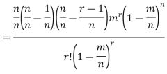
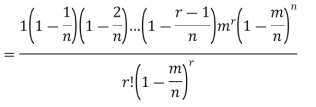
Taking limits when n tends to infinity


MEAN OF POISSON DISTRIBUTION

Success r | Frequency f | f.r |
0 |  | 0 |
1 |  |  |
2 |  |  |
3 |  |  |
… | … | … |
r |  |  |
… | … | … |


STANDARD DEVIATION OF POISSON DISTRIBUTION

Successive r | Frequency f | Product rf | Product  |
0 |  | 0 | 0 |
1 |  |  |  |
2 |  |  |  |
3 |  |  |  |
……. | …….. | …….. | …….. |
r |  |  |  |
…….. | ……. | …….. | ……. |


Hence mean and variance of a Poisson distribution are equal to m. Similarly we can obtain,


MEAN DEVIATION
Show that in a Poisson distribution with unit mean, and the mean deviation about the mean is 2/e times the standard deviation.
Solution.  But mean = 1 i.e. m =1 and S.D. =

r | P (r) | |r-1| | P(r)|r-1| |
0 |  | 1 |  |
1 |  | 0 | 0 |
2 |  | 1 |  |
3 |  | 2 |  |
4 |  | 3 |  |
….. | ….. | ….. | ….. |
r |  | r-1 |  |
 Mean Deviation =


MOMENT GENERATING FUNCTION OF POISSON DISTRIBUTION
Solution. 
Let  be the moment generating function then

CUMULANTS
The cumulant generating function  is given by


Now  cumulant =coefficient of
  in K (t) = m
i.e.  , where r = 1,2,3,…
Mean = 


RECURRENCE FORMULA FOR POISSON DISTRIBUTION
SOLUTION. By Poisson distribution


On dividing (2) by (1) we get


Example. Assume that the probability of an individual coal miner being killed in a mine accident during a year is  . Use appropriate statistical distribution to calculate the probability that in a mine employing 200 miners, there will be at least one fatal accident in a year.
Solution. 


Example. Suppose 3% of bolts made by a machine are defective, the defects occuring at random during production. If bolts are packaged 50 per box, find
(a) Exact probability and
(b) Poisson approximation to it, that a given box will contain 5 defectives.
Solution. 

(a) Hence the probability for 5 defectives bolts in a lot of 50.

(b) To get Poisson approximation m = np =
Required Poisson approximation=
Example. In a certain factory producing cycle tyres, there is a smallchance of 1 in 500 tyres to be defective. The tyres are supplied in lots of 10. Using Poisson distribution, calculate the approximate number of lots containing no defective, one defective and two defective tyres, respectively, in a consignment of 10,000 lots.
Solution. 

S.No. | Probability of defective | Number of lots containing defective |
1. |  |  |
2. |   |  |
3. |   |  |
Normal Distribution-
The concept of normal distribution was given by English mathematician Abraham De Moivre in 1733 but the concrete theory was given by Karl Gauss that is why sometime normal distribution is called Gaussian distribution.
Normal distribution is a continuous distribution. It is a limiting case of binomial distribution.
The probability density function of a normal distribution is given by-

Here 
Where 
Note-
1. If a random variable X follows normal distribution with mean  and variance
  then we can write it as- X
2. If X  , then
  is called standard normal variate with mean 0 and standard deviation 1.
3. The probability density function of standard normal variate Z is given as-

Where 
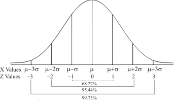
Graph of a normal probability function-
The curve look like bell-shaped curve. The top of the bell is exactly above the mean.
If the value of standard deviation is large then curve tends to flatten out and for small standard deviation it has sharp peak.
This is one of the most important probability distributions in statistical analysis.
Example:
1. If X  then find the probability density function of X.
2. If X  then find the probability density function of X.
Sol.
1. We are given X 
Here 
We know that-

Then the p.d.f. will be-

2. . We are given X 
Here 
We know that-

Then the p.d.f. will be-

Mean, median and mode of the normal distribution-
Let ‘a’ is the median, then it divides the total area into two parts-

Where-

Let a>mean, then-
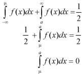
Thus-

So that mean = median.
Note- mean deviation about mean is = 
Mode-
The mode of the normal distribution is  and modal ordinate is given by-

Hence the mean, median and mode are equal in normal distribution.
Area property of a normal distribution (Area under the normal curve)-
Let X follows the normal distribution with mean  and variance
We form a normal curve by taking 
Note- Total area under the curve is always 1.
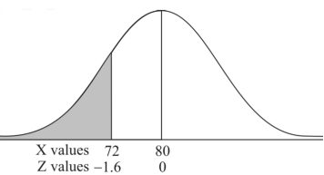
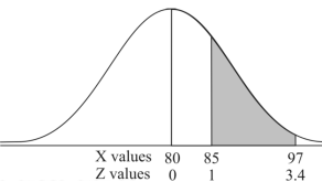
Example: If a random variable X is normally distributed with mean 80 and standard deviation 5, then find-
1. P[X > 95]
2. P[X < 72]
3. P [85 < X <97]
[Note- use the table- area under the normal curve]
Sol.
The standard normal variate is – 
Now-
1. X = 95,

So that-


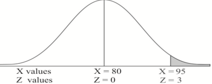
2. X = 72,

So that-


3. X = 85,

X = 97,

So that-


Example: In a company the mean weight of 1000 employees is 60kg and standard deviation is 16kg.
Find the number of employees having their weights-
1. Less than 55kg.
2. More than 70kg.
3. Between 45kg and 65kg.
Sol. Suppose X be a normal variate = the weight of employees.
Here mean 60kg and S.D. = 16kg
X 
Then we know that-

We get from the data,

Now-
1. For X = 55,

So that-
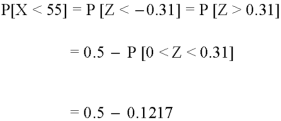

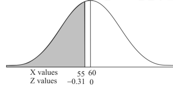
2. For X = 70,

So that-


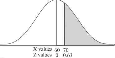
3. For X = 45,

For X = 65,


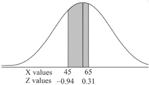
Hence the number of employees having weights between 45kg and 65kg-

Example: The mean inside diameter of a sample of 200 washers produced by a machine is 0.0502 cm and the standard deviation is 0.005 cm. The purpose for which these washers are intended allows a maximum tolerance in the diameter of 0.496 to 0.508 cm, otherwise the washers are considered defective. Determine the percentage of defective washers produced by the machine, assuming the diameters are normally distributed.
Sol.
Here-

And

Area for non-defective washers = area between z = -1.2 to +1.2
= 2 area between z = 0 and z = 1.2
= 2 × 0.3849 = 0.7698 = 76.98%
Then percent of defective washers = 100 – 76.98 = 23.02 %
Example: The life of electric bulbs is normally distributed with mean 8 months and standard deviation 2 months.
If 5000 electric bulbs are issued how many bulbs should be expected to need replacement after 12 months?
[Given that P (z ≥ 2) = 0. 0228]
Sol.
Here mean (μ) = 8 and standard deviation = 2
Number of bulbs = 5000
Total months (X) = 12
We know that-

Area (z ≥ 2) = 0.0228
Number of electric bulbs whose life is more than 12 months ( Z > 12)
= 5000 × 0.0228 = 114
Therefore replacement after 12 months = 5000 – 114 = 4886 electric bulbs.
When two variables are related in such a way that change in the value of one variable affects the value of the other variable, then these two variables are said to be correlated and there is correlation between two variables.
Example- Height and weight of the persons of a group.
The correlation is said to be perfect correlation if two variables vary in such a way that their ratio is constant always.
Scatter diagram-
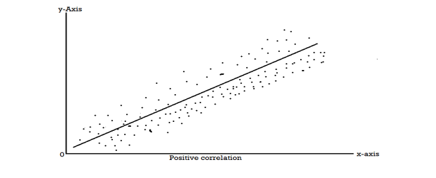
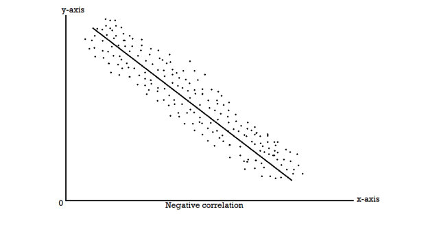
Karl Pearson’s coefficient of correlation-

Here-  and
and 

Note-
1. Correlation coefficient always lies between -1 and +1.
2. Correlation coefficient is independent of change of origin and scale.
3. If the two variables are independent then correlation coefficient between them is zero.
Correlation coefficient | Type of correlation |
+1 | Perfect positive correlation |
-1 | Perfect negative correlation |
0.25 | Weak positive correlation |
0.75 | Strong positive correlation |
-0.25 | Weak negative correlation |
-0.75 | Strong negative correlation |
0 | No correlation |
Example: Find the correlation coefficient between Age and weight of the following data-
Age | 30 | 44 | 45 | 43 | 34 | 44 |
Weight | 56 | 55 | 60 | 64 | 62 | 63 |
Sol.
x | y |  |  |  |  | (   |
30 | 56 | -10 | 100 | -4 | 16 | 40 |
44 | 55 | 4 | 16 | -5 | 25 | -20 |
45 | 60 | 5 | 25 | 0 | 0 | 0 |
43 | 64 | 3 | 9 | 4 | 16 | 12 |
34 | 62 | -6 | 36 | 2 | 4 | -12 |
44 | 63 | 4 | 16 | 3 | 9 | 12 |
Sum= 240 |
360 |
0 |
202 |
0 |
70
|
32 |
Karl Pearson’s coefficient of correlation-

Here the correlation coefficient is 0.27.which is the positive correlation (weak positive correlation), this indicates that the as age increases, the weight also increase.
Short-cut method to calculate correlation coefficient-

Here,


Example: Find the correlation coefficient between the values X and Y of the dataset given below by using short-cut method-
X | 10 | 20 | 30 | 40 | 50 |
Y | 90 | 85 | 80 | 60 | 45 |
Sol.
X | Y |  |  |  |  |  |
10 | 90 | -20 | 400 | 20 | 400 | -400 |
20 | 85 | -10 | 100 | 15 | 225 | -150 |
30 | 80 | 0 | 0 | 10 | 100 | 0 |
40 | 60 | 10 | 100 | -10 | 100 | -100 |
50 | 45 | 20 | 400 | -25 | 625 | -500 |
Sum = 150 |
360 |
0 |
1000 |
10 |
1450 |
-1150 |
Short-cut method to calculate correlation coefficient-


Spearman’s rank correlation-
When the ranks are given instead of the scores, then we use Spearman’s rank correlation to find out the correlation between the variables.
Spearman’s rank correlation coefficient can be defined as-

Example: Compute the Spearman’s rank correlation coefficient of the dataset given below-
Person | A | B | C | D | E | F | G | H | I | J |
Rank in test-1 | 9 | 10 | 6 | 5 | 7 | 2 | 4 | 8 | 1 | 3 |
Rank in test-2 | 1 | 2 | 3 | 4 | 5 | 6 | 7 | 8 | 9 | 10 |
Sol.
Person | Rank in test-1 | Rank in test-2 | d =  |  |
A | 9 | 1 | 8 | 64 |
B | 10 | 2 | 8 | 64 |
C | 6 | 3 | 3 | 9 |
D | 5 | 4 | 1 | 1 |
E | 7 | 5 | 2 | 4 |
F | 2 | 6 | -4 | 16 |
G | 4 | 7 | -3 | 9 |
H | 8 | 8 | 0 | 0 |
I | 1 | 9 | -8 | 64 |
J | 3 | 10 | -7 | 49 |
Sum |
|
|
| 280 |


Regression-
Regression is the measure of average relationship between independent and dependent variable
Regression can be used for two or more than two variables.
There are two types of variables in regression analysis.
1. Independent variable
2. Dependent variable
The variable which is used for prediction is called independent variable.
It is known as predictor or regressor.
The variable whose value is predicted by independent variable is called dependent variable or regressed or explained variable.
The scatter diagram shows relationship between independent and dependent variable, then the scatter diagram will be more or less concentrated round a curve, which is called the curve of regression.
When we find the curve as a straight line then it is known as line of regression and the regression is called linear regression.
Note- regression line is the best fit line which expresses the average relation between variables.
Equation of the line of regression-
Let
y = a + bx ………….. (1)
Is the equation of the line of y on x.
Let  be the estimated value of
  for the given value of
  .
.
So that, According to the principle of least squares, we have the determined ‘a’ and ‘b’ so that the sum of squares of deviations of observed values of y from expected values of y,
That means-

Or
 …….. (2)
Is minimum.
Form the concept of maxima and minima, we partially differentiate U with respect to ‘a’ and ‘b’ and equate to zero.
Which means


And


These equations (3) and (4) are known as normal equation for straight line.
Now divide equation (3) by n, we get-

This indicates that the regression line of y on x passes through the point .
.
We know that-

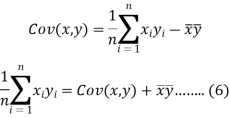
The variance of variable x can be expressed as-


Dividing equation (4) by n, we get-

From the equation (6), (7) and (8)-

Multiply (5) by , we get-

Subtracting equation (10) from equation (9), we get-


Since ‘b’ is the slope of the line of regression y on x and the line of regression passes through the point ( ), so that the equation of the line of regression of y on x is-


This is known as regression line of y on x.
Note-
 are the coefficients of regression.
2. 
Example: Two variables X and Y are given in the dataset below, find the two lines of regression.
x | 65 | 66 | 67 | 67 | 68 | 69 | 70 | 71 |
y | 66 | 68 | 65 | 69 | 74 | 73 | 72 | 70 |
Sol.
The two lines of regression can be expressed as-

And

x | y |  |  | Xy |
65 | 66 | 4225 | 4356 | 4290 |
66 | 68 | 4356 | 4624 | 4488 |
67 | 65 | 4489 | 4225 | 4355 |
67 | 69 | 4489 | 4761 | 4623 |
68 | 74 | 4624 | 5476 | 5032 |
69 | 73 | 4761 | 5329 | 5037 |
70 | 72 | 4900 | 5184 | 5040 |
71 | 70 | 5041 | 4900 | 4970 |
Sum = 543 | 557 | 36885 | 38855 | 37835 |
Now-

And

Standard deviation of x-


Similarly-


Correlation coefficient-


Put these values in regression line equation, we get
Regression line y on x-


Regression line x on y-


Regression line can also be find by the following method-
Example: Find the regression line of y on x for the given dataset.
X | 4.3 | 4.5 | 5.9 | 5.6 | 6.1 | 5.2 | 3.8 | 2.1 |
Y | 12.6 | 12.1 | 11.6 | 11.8 | 11.4 | 11.8 | 13.2 | 14.1 |
Sol.
Let y = a + bx is the line of regression of y on x, where ‘a’ and ‘b’ are given as-


We will make the following table-
x | y | Xy |  |
4.3 | 12.6 | 54.18 | 18.49 |
4.5 | 12.1 | 54.45 | 20.25 |
5.9 | 11.6 | 68.44 | 34.81 |
5.6 | 11.8 | 66.08 | 31.36 |
6.1 | 11.4 | 69.54 | 37.21 |
5.2 | 11.8 | 61.36 | 27.04 |
3.8 | 13.2 | 50.16 | 14.44 |
2.1 | 14.1 | 29.61 | 4.41 |
Sum = 37.5 | 98.6 | 453.82 | 188.01 |
Using the above equations we get-


On solving these both equations, we get-
a = 15.49 and b = -0.675
So that the regression line is –
y = 15.49 – 0.675x
Note – Standard error of predictions can be find by the formula given below-

Difference between regression and correlation-
1. Correlation is the linear relationship between two variables while regression is the average relationship between two or more variables.
2. There are only limited applications of correlation as it gives the strength of linear relationship while the regression is to predict the value of the dependent varibale for the given values of independent variables.
3. Correlation does not consider dependent and independent variables while regression consider one dependent variable and other indpendent variables.
RANK CORRELATION
A group of n individuals may be arranged in order to merit with respect to some characteristics. The same group would give different orders for different characteristics. Considering the orders corresponding to two characteristics A and B, the correction between these n pairs of rank is called the rank correlation in the characteristics A and B for that group of individuals.
Let  be the ranks of the ith individuals in A and B respectively. Assuming that no two individuals are bracketed equal in either case, each of the variables taking the values 1,2,3,…,n we have

If X, Y be the deviations of x, y from their means, then


Now let, 


Hence the correlation coefficient between these variables is

This is called the rank correlation coefficient and is denoted by 
Example. Ten participants in a contest are ranked by two judges as follows:
x | 1 | 6 | 5 | 10 | 3 | 2 | 4 | 9 | 7 | 8 |
y | 6 | 4 | 9 | 8 | 1 | 2 | 3 | 10 | 5 | 7 |
Calculate the rank correlation coefficient 
Solution. If 

Hence, 
Example. Three judges A,B,C give the following ranks. Find which pair of judges has common approach
A | 1 | 6 | 5 | 10 | 3 | 2 | 4 | 9 | 7 | 8 |
B | 3 | 5 | 8 | 4 | 7 | 10 | 2 | 1 | 6 | 9 |
C | 6 | 4 | 9 | 8 | 1 | 2 | 3 | 10 | 5 | 7 |
Solution. Here n = 10
A (=x) | Ranks by B(=y) | C (=z) |  x-y |  y - z |  z-x | 
|  |  |
1 | 3 | 6 | -2 | -3 | 5 | 4 | 9 | 25 |
6 | 5 | 4 | 1 | 1 | -2 | 1 | 1 | 4 |
5 | 8 | 9 | -3 | -1 | 4 | 9 | 1 | 16 |
10 | 4 | 8 | 6 | -4 | -2 | 36 | 16 | 4 |
3 | 7 | 1 | -4 | 6 | -2 | 16 | 36 | 4 |
2 | 10 | 2 | -8 | 8 | 0 | 64 | 64 | 0 |
4 | 2 | 3 | 2 | -1 | -1 | 4 | 1 | 1 |
9 | 1 | 10 | 8 | -9 | 1 | 64 | 81 | 1 |
7 | 6 | 5 | 1 | 1 | -2 | 1 | 1 | 4 |
8 | 9 | 7 | -1 | 2 | -1 | 1 | 4 | 1 |
Total |
|
| 0 | 0 | 0 | 200 | 214 | 60 |


Method of Least Squares
Let  (1)
(1)
Be the straight line to be fitted to the given data points

Let  be the theoretical value for
Then, 


For S to be minimum


On simplification equation (2) and (3) becomes


The equation (3) and (4) are known as Normal equations.
On solving ( 3) and (4) we get the values of a and b
(b)To fit the parabola

The normal equations are 


On solving three normal equations we get the values of a,b and c.
Example. Find the best values of a and b so that y = a + bx fits the data given in the table
x | 0 | 1 | 2 | 3 | 4 |
y | 1.0 | 2.9 | 4.8 | 6.7 | 8.6 |
Solution.
y = a + bx
x | y | Xy |  |
0 | 1.0 | 0 | 0 |
1 | 2.9 | 2.0 | 1 |
2 | 4.8 | 9.6 | 4 |
3 | 6.7 | 20.1 | 9 |
4 | 8.6 | 13.4 | 16 |
 |  |  |  |
Normal equations,  y= na+ b
 x (2)
x (2)

On putting the values of 


On solving (4) and (5) we get,

On substituting the values of a and b in (1) we get

Example. By the method of least squares, find the straight line that best fits the following data :
x | 1 | 2 | 3 | 4 | 5 |
y | 14 | 27 | 40 | 55 | 68 |
Solution. Let the equation of the straight line best fit be y = a + bx. (1)
x | y | x y |  |
1 | 14 | 14 | 1 |
2 | 27 | 54 | 4 |
3 | 40 | 120 | 9 |
4 | 55 | 220 | 16 |
5 | 68 | 340 | 25 |
 |  |  |  |
Normal equations are 

On putting the values of  x,
x,  y,
y,  xy and
  in (2) and (3) we have


On solving equations (4) and (5) we get

On substituting the values of (a) and (b) in (1) we get,

Example. Find the least squares approximation of second degree for the discrete data
x | 2 | -1 | 0 | 1 | 2 |
y | 15 | 1 | 1 | 3 | 19 |
Solution. Let the equation of second degree polynomial be 
x | y | Xy |  |  |  |  |
-2 | 15 | -30 | 4 | 60 | -8 | 16 |
-1 | 1 | -1 | 1 | 1 | -1 | 1 |
0 | 1 | 0 | 0 | 0 | 0 | 0 |
1 | 3 | 3 | 1 | 3 | 1 | 1 |
2 | 19 | 38 | 4 | 76 | 8 | 16 |
 |  |  |  |  |  |  |
Normal equations are 


On putting the values of  x,
x,  y,
y, xy,
xy,  have
have


On solving (5),(6),(7), we get, 
The required polynomial of second degree is

Second degree parabolas and more general curves
Change of scale
If the data is of equal interval in large numbers then we change the scale as 
Example. Fit a second degree parabola to the following data by least square method:
x | 1929 | 1930 | 1931 | 1932 | 1933 | 1934 | 1935 | 1936 | 1937 |
y | 352 | 356 | 357 | 358 | 360 | 361 | 365 | 360 | 359 |
Solution. Taking 
Taking 

The equation  is transformed to
x |  | y |  | Uv |  |  |  |  |
1929 | -4 | 352 | -5 | 20 | 16 | -80 | -64 | 256 |
1930 | -3 | 360 | -1 | 3 | 9 | -9 | -27 | 81 |
1931 | -2 | 357 | 0 | 0 | 4 | 0 | -8 | 16 |
1932 | -1 | 358 | 1 | -1 | 1 | 1 | -1 | 1 |
1933 | 0 | 360 | 3 | 0 | 0 | 0 | 0 | 0 |
1934 | 1 | 361 | 4 | 4 | 1 | 4 | 1 | 1 |
1935 | 2 | 361 | 4 | 8 | 4 | 16 | 8 | 16 |
1936 | 3 | 360 | 3 | 9 | 9 | 27 | 27 | 81 |
1937 | 4 | 350 | 2 | 8 | 16 | 32 | 64 | 256 |
Total |
 |
|  |  |  |  |  |  |
Normal equations are


On solving these equations we get 


Example. Fit a second degree parabola to the following data.
x=1.0 | 1.5 | 2.0 | 2.5 | 3.0 | 3.5 | 4.0 |
y=1.1 | 1.3 | 1.6 | 2.0 | 2.7 | 3.4 | 4.1 |
Solution. We shift the origin to (2.5, 0) antique 0.5 as the new unit. This amounts to changing the variable x to X, by the relation X = 2x – 5.
Let the parabola of fit be y = a + bX  The values of
  X etc. Are calculated as below:
x | X | y | Xy |  |  |  |  |
1.0 | -3 | 1.1 | -3.3 | 9 | 9.9 | -27 | 81 |
1.5 | -2 | 1.3 | -2.6 | 4 | 5.2 | -5 | 16 |
2.0 | -1 | 1.6 | -1.6 | 1 | 1.6 | -1 | 1 |
2.5 | 0 | 2.0 | 0.0 | 0 | 0.0 | 0 | 0 |
3.0 | 1 | 2.7 | 2.7 | 1 | 2.7 | 1 | 1 |
3.5 | 2 | 3.4 | 6.8 | 4 | 13.6 | 8 | 16 |
4.0 | 3 | 4.1 | 12.3 | 9 | 36.9 | 27 | 81 |
Total | 0 | 16.2 | 14.3 | 28 | 69.9 | 0 | 196 |
The normal equations are
7a + 28c =16.2; 28b =14.3;. 28a +196c=69.9
Solving these as simultaneous equations we get


Replacing X bye 2x – 5 in the above equation we get

Which simplifies to y = This is the required parabola of the best fit.