Unit – 4

Matrices

4.1 Rank of a matrix (Echelon form and Normal form)

Definition:

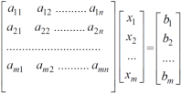
An arrangement of m.n numbers in m rows and n columns is called a matrix of order mxn.

Generally a matrix is denoted by capital letters. Like, A, B, C, ….. Etc.

Types of matrices:- (Review)

1. Row matrix
2. Column matrix
3. Square matrix
4. Diagonal matrix
5. Trace of a matrix
6. Determinant of a square matrix
7. Singular matrix
8. Non – singular matrix
9. Zero/ null matrix
10. Unit/ Identity matrix
11. Scaler matrix
12. Transpose of a matrix
13. Triangular matrices
14. Upper triangular and lower triangular matrices,
15. Conjugate of a matrix
16. Symmetric matrix
17. Skew – symmetric matrix

Operations on matrices:

1. Equality of two matrices
2. Multiplication of A by a scalar k.
3. Addition and subtraction of two matrices
4. Product of two matrices
5. Inverse of a matrix

Elementary transformations

a)     Elementary row transformation

These are three elementary transformations

1. Interchanging any two rows (Rij)
2. Multiplying all elements in ist row by a non – zero constant k is denoted by KRi
3. Adding to the elements in ith row by the kth multiple of jth row is denoted by .

b)    Elementary column transformations:

There are three elementary column transformations.

1. Interchanging ith and jth column. Is denoted by Cij.
2. Multiplying ith column by a non – zero constant k is denoted by kCj.
3. Adding to the element of ith column by the kth multiple of jth column is denoted by Ci + kCj.

Elementary transformation

A matrix can be transformed to another matrix by performing certain operations, we call these operations as elementary row operations and elementary column operations.

Definition-

“Two matrices A and B of same order are said to be equivalent to one another if one can be obtained from the other by the applications of elementary transformations.”

Note-

1. A ~ B to mean that the matrix A is equivalent to the matrix B.
2. An elementary transformation transforms a given matrix into another matrix which need not be equal to the given matrix.

Elementary row and column operations-

1. The interchanging of any two rows or columns of the matrix
2. Replacing a row or column of the matrix by a non-zero scalar multiple of the row (column) by a non-zero scalar.
3. Replacing a row or column of the matrix by a sum of the row (column) with a non-zero scalar multiple of another row or column of the matrix.

Notations for elementary row transformations:

Interchanging of and rows is denoted by↔

The multiplication of each element of row by a non-zero constant λis denoted by

Using the row elementary operations, we can transform a given non-zero matrix to a simplified form called a Row-echelon form.

In a row-echelon form, we may have rows all of whose entries are zero. Such rows are called zero rows. A non-zero row is one in which at least one of the entries is not zero.

A non-zero matrix is in a row-echelon form if all zero rows occur as bottom rows of the matrix, and if the first non-zero element in any lower row occurs to the right of the first non-zero entry in the higher row.

Definition-A non-zero matrix A is said to be in a row-echelon form if:

1. All zero rows of A occur below every non-zero row of A.
2. The first non-zero element in any row i of E occurs in the column of A, then all other entries in the column of A below the first non-zero element of row i are zeros.
3. The first non-zero entry in the row of A lies to the left of the first non-zero entry in (row of A.

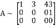
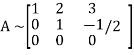
Example: Reduce the following matrix into row-echelon form-

Sol.

We have-

Apply-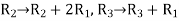

Apply-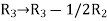

Rank of a matrix-

Rank of a matrix by echelon form-

The rank of a matrix (r) can be defined as –

1. It has at least one non-zero minor of order r.

2. Every minor of A of order higher than r is zero.

Example: Find the rank of a matrix M  by echelon form.

M = 

Sol. First we will convert the matrix M into echelon form,

M =

Apply, , we get

M =

Apply  , we get

M =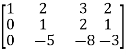

Apply 

M =

We can see that, in this echelon form of matrix, the number of non – zero rows is 3.

So that the rank of matrix X will be 3.

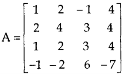
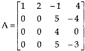
Example: Find the rank of a matrix A by echelon form.

A =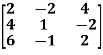

Sol. Convert the matrix A into echelon form,

A =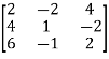

Apply 

A =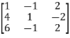

Apply 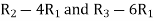   , we get

A =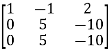

Apply , we get

A =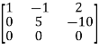

Apply ,

A =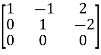

Apply  ,

A =

Therefore the rank of the matrix will be 2.

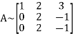
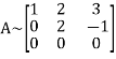
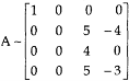
Example:  Find the rank of a matrix A by echelon form.

A =

Sol. Transform the matrix A into echelon form, then find the rank,

We have,

A =

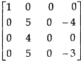
Apply, 

A =

Apply ,

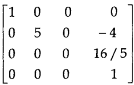
A =

Apply

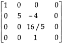
A =

Apply

A =

Hence the rank of the matrix will be 2.

Example:  Find the rank of the following matrices by echelon form?

Let A =

Applying

A 

Applying

A 

Applying

A 

Applying

A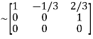 

It is  clear  that  minor  of order 3  vanishes but  minor  of order  2  exists  as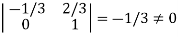 

Hence rank of a given matrix A is 2 denoted by 

2.    

Let  A  = 

Applying

Applying

Applying

The minor of order 3 vanishes but minor of order 2 non zero as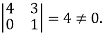 

Hence the rank of matrix A is 2 denoted by

3.    

Let A =

Apply

Apply

Apply

It is clear that the minor of order 3 vanishes where as the minor of order 2 is non zero as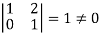 

Hence the rank of given matrix is 2 i.e.

Echelon form and Normal form

Rank of a matrix by normal form-

Any matrix ‘A’ which is non-zero can be reduced to a normal form of ‘A’ by using elementary transformations.

There are 4 types of normal forms –

The number r obtained is known as rank of matrix A.

Both row and column transformations may be used in order to find the rank of the matrix.

Note-Normal form is also known as canonical form

Example: Reduce the following matrix to normal form of Hence find it’s rank,

Solution:

We have,

Apply

• Rank of A = 1

Example: Find the rank of the matrix

Solution:

We have,

Apply R12

• Rank of A = 3

Example: Find the rank of the following matrices by reducing it to the normal form.

Solution:

Apply C14

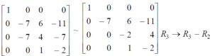
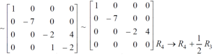
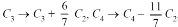
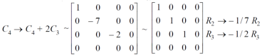
Example: reduce the matrix A to its normal form and find rank as well.

Sol.  We have,

We will apply elementary row operation,

We get,

Now apply column transformation,

We get,

Apply

  , we get,

Apply   and

Apply 

Apply   and

Apply   and

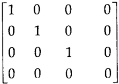
As we can see this is required normal form of matrix A.

Therefore the rank of matrix A is 3.

Example: Find the rank of a matrix A by reducing into its normal form.

Sol.  We are given,

Apply

Apply

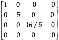
This is the normal form of matrix A.

So that the rank of matrix A = 3

Key takeaways-

1. There are 4 types of normal forms –

2.     Normal form is also known as canonical form

4.2 System of linear Equations(consistency and inconsistency)

There are two types of linear equations-

1.  Consistent                                   

2. Inconsistent

Let’s understand about these two types of linear equations.

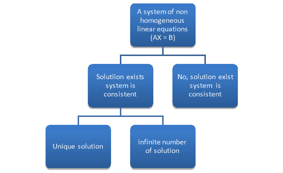
Consistent –

If a system of equations has one or more than one solution, it is said be consistent.

There could be unique solution or infinite solution.

For example-

A system of linear equations-

2x + 4y = 9

x + y = 5

Has unique solution,

Whereas,

A system of linear equations-

2x + y = 6

4x + 2y = 12

Has infinite solutions.

Inconsistent-

If a system of equations has no solution, then it is called inconsistent.

Consistency of a system of linear equations-

Suppose that a system of linear equations is given as-

This is the format as AX = B

Its augmented matrix is-

[A:B] = C

(1) Consistent equations-

If Rank of A = Rank of C

Here, Rank of A = Rank of C = n ( no. Of unknown) – unique solution

And Rank of A = Rank of C = r , where r<n   -  infinite solutions

(2) Inconsistent equations-

If Rank of A ≠ Rank of C

Solution of homogeneous system of linear equations-

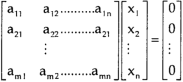
A system of linear equations of the form AX = O is said to be homogeneous, where A denotes the coefficients and of matrix and O denotes the null vector.

Suppose the system of homogeneous linear equations is,

It means ,

AX = O

Which can be written in the form of matrix as below,

Note-  A system of homogeneous linear  equations always has a solution if

1. r(A) = n then there will be trivial solution, where n is the number of unknown,

2. r(A) <n , then there will be an infinite number of solution.

Example: Find the solution of the following homogeneous system of linear equations,

Sol. The given system of linear equations can be written in the form of matrix as follows,

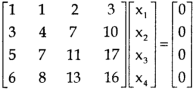
Apply the elementary row transformation,

  , we get,

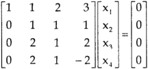
    , we get

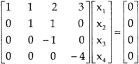
Here r(A) = 4, so that it has trivial solution,

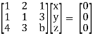
Example: Find out the value of ‘b’ in the system of homogenenous equations-

2x + y + 2z = 0

x + y + 3z = 0

4x + 3y +  bz = 0

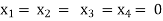
Which has

(1) Trivial solution

(2) Non-trivial solution

Sol. (1)

For trivial solution, we already know that the values of x , y and z will be zerp, so that ‘b’ can have any value.

Now for non-trivial solution-

(2)

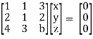
Convert the system of equations into matrix form-

AX = O

Apply Respectively , we get the following resultant matrices

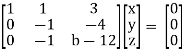
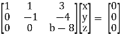
For non-trivial solutions, r(A) = 2 < n

b – 8 = 0

b = 8

Solution of non-homogeneous system of linear equations-

Example-1: check whether the following system of linear equations is consistent of not.

2x + 6y = -11

6x + 20y – 6z = -3

6y – 18z = -1

Sol. Write the above system of linear equations in augmented matrix form,

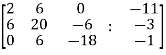
Apply , we get

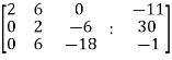
Apply

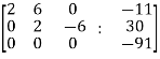
Here the rank of C is 3 and the rank of A is 2

Therefore both ranks are not equal. So that the given system of linear equations is not consistent.

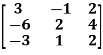
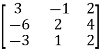
Example: Check the consistency and find the values of x , y and z of the following system of linear equations.

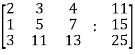
2x + 3y + 4z = 11

X + 5y + 7z = 15

3x + 11y + 13z = 25

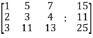
Sol. Re-write the system of equations in augmented matrix form.

C = [A,B]

That will be,

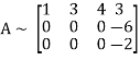
Apply 

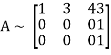
Now apply ,

We get,

~~

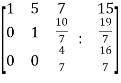
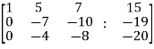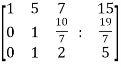Here rank of A = 3

And rank of C = 3, so that the system of equations is consistent,

So that we can can solve the equations as below,

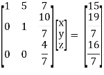
That gives,

x + 5y + 7z = 15  ……………..(1)

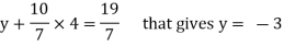
y + 10z/7 = 19/7 ………………(2)

4z/7 = 16/7 ………………….(3)

From eq. (3)

z = 4,

From 2,

From eq.(1), we get

x + 5(-3) + 7(4) = 15

That gives,

x = 2

Therefore the values of x , y , z are    2 , -3 , 4  respectively. 

4.3Eigenvalues and Eigenvectors

Introduction:

In this chapter we are going to study a very important theorem viz first we have to study of eigen values and eigen vector.

1. Vector

An ordered n – touple of numbers is called an n – vector. Thus the ‘n’ numbers x1, x2, ………… xn taken in order denote the vector x. i.e. x = (x1, x2, ……., xn).

Where the numbers x1, x2, ……….., xn are called component or co – ordinates of a vector x. A vector may be written as row vector or a column vector.

If A be anmxn matrix then each row will be an n – vector & each column will be an m – vector.

2.     Linear Dependence

A set of n – vectors. x1, x2, …….., xr is said to be linearly dependent if there exist scalars. k1, k2, ……., kr not all zero such that

k1 + x2k2 + …………….. + xrkr = 0     … (1)

3.     Linear Independence

A set of r vectors x1, x2, …………., xr is said to be linearly independent if there exist scalars k1, k2, …………, kr all zero such that

x1 k1 + x2 k2 + …….. + xrkr = 0

Note:-

1. Equation (1) is known as a vector equation.
2. If the vector equation has non – zero solution i.e. k1, k2, …., kr not all zero. Then the vector x1, x2, ………. xr are said to be linearly dependent.
3. If the vector equation has only trivial solution i.e.

k1 = k2 = …….=kr = 0. Then the vector x1, x2, ……, xr are said to linearly independent.

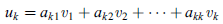
4.     Linear combination

A vector x can be written in the form.

x = x1 k1 + x2 k2 + ……….+xrkr

Where k1, k2, ………….., kr are scalars, then X is called linear combination of x1, x2, ……, xr.

Results:

1. A set of two or more vectors are said to be linearly dependent if at least one vector can be written as a linear combination of the other vectors.
2. A set of two or more vector are said to be linearly independent then no vector can be expressed as linear combination of the other vectors.

Example 1

Are the vectors , , linearly dependent. If so, express x1 as a linear combination of the others.

Solution:

Consider a vector equation,

i.e.

Which can be written in matrix form as,

Here & no. Of unknown 3. Hence the system has infinite solutions. Now rewrite the questions as,

Put

and

Thus

i.e.

i.e.

Since F11 k2, k3 not all zero. Hence are linearly dependent.

Example 2

Examine whether the following vectors are linearly independent or not.

and .

Solution:

Consider the vector equation,

i.e.  … (1)

Which can be written in matrix form as,

R12

R2 – 3R1, R3 – R1

R3 + R2

Here Rank of coefficient matrix is equal to the no. Of unknowns. i.e. r = n = 3.

Hence the system has unique trivial solution.

i.e.

i.e. vector equation (1) has only trivial solution. Hence the given vectors x1, x2, x3 are linearly independent.

Example 3

At what value of P the following vectors are linearly independent.

Solution:

Consider the vector equation.

i.e.

This is a homogeneous system of three equations in 3 unknowns and has a unique trivial solution.

If and only if Determinant of coefficient matrix is non zero.

consider .

.

i.e.

Thus for the system has only trivial solution and Hence the vectors are linearly independent.

Note:

If the rank of the coefficient matrix is r, it contains r linearly independent variables & the remaining vectors (if any) can be expressed as linear combination of these vectors.

Characteristic equation:

Let A he a square matrix, be any scaler then is called characteristic equation of a matrix A.

Note:

Let a be a square matrix and ‘’ be any scaler then,

1)     is called characteristic matrix

2)     is called characteristic polynomial.

The roots of a characteristic equations are known as characteristic root or latent roots, eigen values or proper values of a matrix A.

Eigen vector:

Suppose be an eigen value of a matrix A. Then a non – zero vector x1 such that.

     … (1)

Such a vector ‘x1’ is called as eigen vector corresponding to the eigen value .

Properties of Eigen values:

1. Then sum of the eigen values of a matrix A is equal to sum of the diagonal elements of a matrix A.
2. The product of all eigen values of a matrix A is equal to the value of the determinant.
3. If are n eigen values of square matrix A then are m eigen values of a matrix A-1.
4. The eigen values of a symmetric matrix are all real.
5. If all eigen values are non – zen then A-1 exist and conversely.
6. The eigen values of A and A’ are same.

Properties of eigen vector:

1. Eigen vector corresponding to distinct eigen values are linearly independent.
2. If two are more eigen values are identical then the corresponding eigen vectors may or may not be linearly independent.
3. The eigen vectors corresponding to distinct eigen values of a real symmetric matrix are orthogonal.

Example 1

Determine the eigen values of eigen vector of the matrix.

Solution:

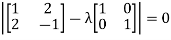
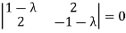
Consider the characteristic equation as,

i.e.

i.e.

i.e.

Which is the required characteristic equation.

are the required eigen values.

Now consider the equation

        … (1)

Case I:

If   Equation (1) becomes

R1 + R2

Thus

independent variable.

Now rewrite equation as,

Put x3 = t

&

Thus .

Is the eigen vector corresponding to .

Case II:

If equation (1) becomes,

Here

independent variables

Now rewrite the equations as,

Put

&

.

Is the eigen vector corresponding to .

Case III:

If equation (1) becomes,

Here rank of

independent variable.

Now rewrite the equations as,

Put

Thus .

Is the eigen vector for .

Example 2

Find the eigen values of eigen vector for the matrix.

Solution:

Consider the characteristic equation as

i.e.

i.e.

are the required eigen values.

Now consider the equation

       … (1)

Case I:

Equation (1) becomes,

Thus and n = 3

3 – 2 = 1 independent variables.

Now rewrite the equations as,

Put

,

i.e. the eigen vector for

Case II:

If equation (1) becomes,

Thus

Independent variables.

Now rewrite the equations as,

Put

Is the eigen vector for

Now

Case II:

If equation (1) gives,

R1 – R2

Thus

 independent variables

Now

Put

Thus

Is the eigen vector for .

4.4 Diagonalization ofsquare matrices

Two square matrix and A of same order n are said to be similar if and only if

for some non singular matrix P.

Such transformation of the matrix A into with the help of non singular matrix P is known as similarity transformation.

Similar matrices have the same Eigen values.

If X is an Eigen vector of matrix A then is Eigen vector of the matrix

Reduction to Diagonal Form:

Let A be a square matrix of order n has n linearly independent Eigen vectors which form the  matrix P such that

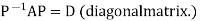
Where P is called the modal matrix and D is known as spectral matrix.

Procedure: let A be a square   matrix of order 3.

Let three Eigen vectors of A are 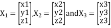 corresponding to Eigen values

Let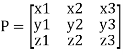     

  {by characteristics equation of A}

Or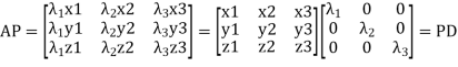

Or 

Note: The method of diagonalization is helpful in calculating power of a matrix.

.Then for an integer n we have  

We are using the example of 1.6*

Example1:  Diagonalise the matrix

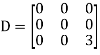
Let A=

The three Eigen vectors obtained are  (-1,1,0), (-1,0,1) and (3,3,3) corresponding to Eigen values .

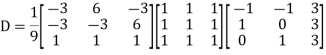
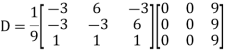
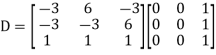
Then 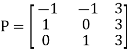   and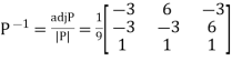

Also we know that    

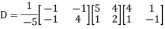
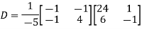
Example2: Diagonalise the matrix

Let A =

The Eigen vectors are (4,1),(1,-1) corresponding to Eigen values .

Then    and also 

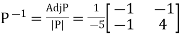
Also we know that    

4.5Cayley-Hamilton Theorem

Statement-

Every square matrix satisfies its characteristic equation, that means for every square matrix of order n,

|A - | =

Then the matrix equation-

Is satisfied by X = A

That means

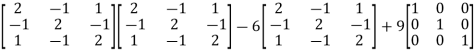
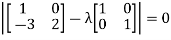
Example-1: Find the characteristic equation of the matrix A =   and verify cayley-Hamlton theorem.

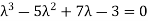
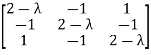
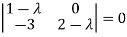
Sol. Characteristic equation of the matrix, we can be find as follows-

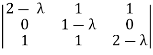
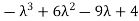
Which is,

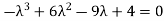
( 2 -  , which gives

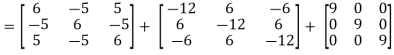
According to cayley-Hamilton theorem,

  …………(1)

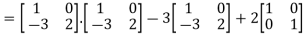
Now we will verify equation (1),

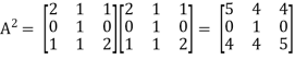
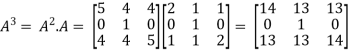
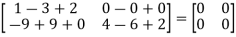
Put the required values in equation (1) , we get

Hence the cayley-Hamilton theorem is verified.

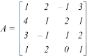
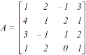
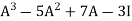
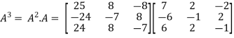
Example-2: Find the characteristic equation of the the matrix A and verify Cayley-Hamilton theorem as well.

A =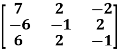

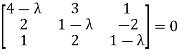
Sol. Characteristic equation will be-

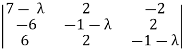= 0

( 7 -

(7-

(7-

Which gives,

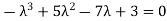
Or

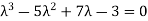
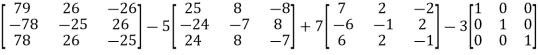
According to cayley-Hamilton theorem,

   …………………….(1)

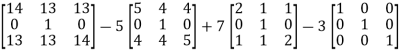
In order to verify cayley-Hamilton theorem , we will find the values of 

So that,

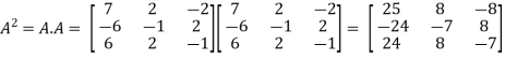
Now

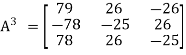
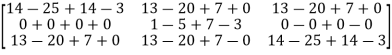
Put these values in equation(1), we get

= 0

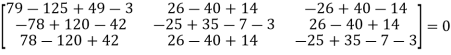
Hence the cayley-hamilton theorem is verified.

Example-3:Using Cayley-Hamilton theorem, find , if A = ?

Sol. Let A =

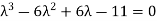
The characteristics equation of A is

Or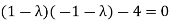

Or

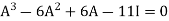
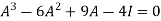
By Cayley-Hamilton theorem   

L.H.S.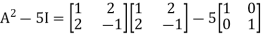

=

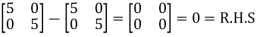
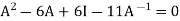
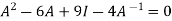
By Cayley-Hamilton theorem we have   

Multiply both side by

.

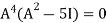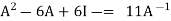
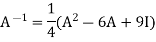
Or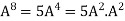 

=

=

Inverse of a matrix by Cayley-Hamilton theorem-

We can find the inverse of any matrix by multiplying the characteristic equation With.

For example, suppose we have a characteristic equation 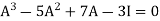  then multiply this by  , then it becomes

Then we can find by solving the above equation.

Example-1: Find the inverse of matrix A by using Cayley-Hamilton theorem.

A =

Sol.  The characteristic equation will be,

|A - | = 0

Which gives,

(4-

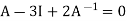
According to Cayley-Hamilton theorem,

Multiplying by 

That means

On solving,

11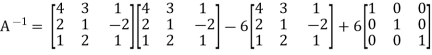

= 

= 

So that,

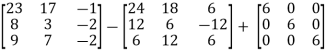
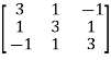
Example-2: Find the inverse of matrix A by using Cayley-Hamilton theorem.

A =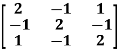

Sol.  The characteristic equation will be,

|A - | = 0

= 

= (2-

= (2 -

=

That is,

Or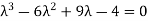
 

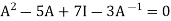
We know that by Cayley-Hamilton theorem,

…………………….(1)t,

Multiply equation(1) by , we get

Or

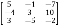
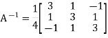
Now we will find 

=

=

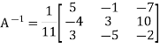
Hence the inverse of matrix A is,

Example-3: Verify the Cayley-Hamilton theorem and find the inverse.

?

Sol.  Let A =

The characteristics equation of A is

Or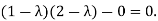

Or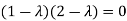 

Or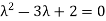 

By Cayley-Hamilton theorem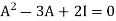 

L.H.S:

=   =0=R.H.S

Multiply both side by on 

Or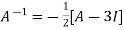

Or [

Or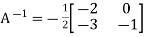

4.6 Inner product spaces

Definition: Let V be a vector space over F. An inner product on V

Is a function that assigns, to every ordered pair of vectors x and y in V, a scalar in F, denoted , such that for all x, y, and z in V and all c in F, the following hold:

(a)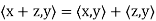 

(b)

(c) 

(d)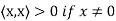

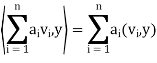
Note that (c) reduces to = if F = R. Conditions (a) and (b) simply require that the inner product be linear in the first component.

It is easily shown that if and , then

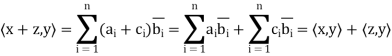
Example: For x = () and y = () in , define

The verification that satisfies conditions (a) through (d) is easy. For example, if z = () we have for (a)

Thus, for x = (1+i, 4) and y = (2 − 3i,4 + 5i) in

A vector space V over F endowed with a specific inner product is called an inner product space. If F = C, we call V a complex inner product It is clear that if V has an inner product and W is a subspace of

V, then W is also an inner product space when the same function is

Restricted to the vectors x, y ∈ W.space, whereas if F = R, we call V a real inner product space.

Theorem: Let V be an inner product space. Then for x, y, z ∈ V and c ∈ F, the following statements are true.

(a)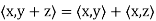 

(b)

(c) 

(d)

(e)  If

Note- Let V be an inner product space. For x ∈ V, we define the norm or length of x is given by ||x|| =

4.7 Gram-Schmidt orthogonalization(process)

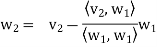
Suppose {} is a basis of an inner product space V. One can use this basis to construct an orthogonal basis {} of V as follows. Set

………………

……………….
 

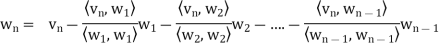
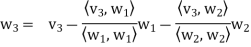
In other words, for k = 2, 3, . . . , n, we define

Where

Is the component of .

Each is orthogonal to the preceeding w’s. Thus, form an orthogonal basis for V as claimed. Normalizing each wi will then yield an orthonormal basis for V.

The above process is known as the Gram–Schmidt orthogonalization process.

Note-

1. Each vector wk is a linear combination of and the preceding w’s. Hence, one can easily show, by induction, that each is a linear combination of
2. Because taking multiples of vectors does not affect orthogonality, it may be simpler in hand calculations to clear fractions in any new  , by multiplying  by an appropriate scalar, before obtaining the next .

Theorem: Let be any basis of an inner product space V. Then there exists an orthonormal basis of V such that the change-of-basis matrix from { to { is triangular; that is, for k = 1; . . . ; n,

Theorem: Suppose S = is an orthogonal basis for a subspace W of a vector space V. Then one may extend S to an orthogonal basis for V; that is, one may find vectors , such that  is an orthogonal basis for V.

Example: Apply the Gram–Schmidt orthogonalization process to find an orthogonal basis and then an orthonormal basis for the subspace U of spanned by

Sol:

Step-1: First  =

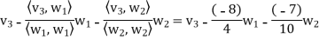
Step-2: Compute

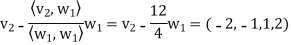
Now set-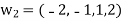

Step-3: Compute

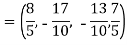
Clear fractions to obtain,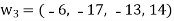

Thus, , , form an orthogonal basis for U. Normalize these vectors to obtain an orthonormal basis

of U. We have

So

References:

1. D. Poole, “Linear Algebra: A Modern Introduction”, Brooks/Cole, 2005.
2. N.P. Bali and M. Goyal, “A Text Book of Engineering Mathematics”, Laxmi Publications, 2008.
3. B.S. Grewal, “Higher Engineering Mathematics”, Khanna Publishers, 2010.
4. V. Krishnamurthy, V. P. Mainra and J. L. Arora, “An Introduction to Linear Algebra”, Affiliated East-West Press, 2005.
5. G.B. Thomas and R.L. Finney, “Calculus and Analytic Geometry”, Pearson, 2002.