Unit - 3

Special Search Techniques

3.1 Heuristic search

Heuristics function: Heuristic is a function which is used in Informed Search, and it finds the most promising path. It takes the current state of the agent as its input and produces the estimation of how close agent is from the goal. The heuristic method, however, might not always give the best solution, but it guaranteed to find a good solution in reasonable time. Heuristic function estimates how close a state is to the goal. It is represented by h(n), and it calculates the cost of an optimal path between the pair of states. The value of the heuristic function is always positive.

Admissibility of the heuristic function is given as:

h(n) <= h*(n)  

Here h(n) is heuristic cost, and h*(n) is the estimated cost. Hence heuristic cost should be less than or equal to the estimated cost.

Pure Heuristic Search:

Pure heuristic search is the simplest form of heuristic search algorithms. It expands nodes based on their heuristic value h(n). It maintains two lists, OPEN and CLOSED list. In the CLOSED list, it places those nodes which have already expanded and in the OPEN list, it places nodes which have yet not been expanded.

On each iteration, each node n with the lowest heuristic value is expanded and generates all its successors and n is placed to the closed list. The algorithm continues unit a goal state is found.

In the informed search we will discuss two main algorithms which are given below:

●        Best First Search Algorithm(Greedy search)

●        A* Search Algorithm

Key takeaway

Heuristic is a function which is used in Informed Search, and it finds the most promising path. It takes the current state of the agent as its input and produces the estimation of how close agent is from the goal.

3.2 Greedy best

The technique of this method is very similar to that of the best first search algorithm. It's a simple best-first search that reduces the expected cost of accomplishing the goal. It basically chooses the node that appears to be closest to the goal. Before assessing the change in the score, this search starts with the initial matrix and makes all possible adjustments. The modification is then applied until the best result is achieved. The search will go on until no further improvements can be made. A lateral move is never made by the greedy search.

It reduces the search time by using the least estimated cost h (n) to the goal state as a measure, however the technique is neither comprehensive nor optimal. The key benefit of this search is that it is straightforward and results in speedy results. The downsides include the fact that it is not ideal and is prone to false starts.

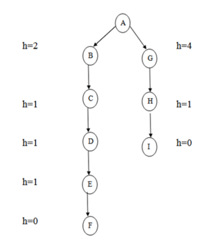
Fig 1: Greedy search

The best first search algorithm is a graph search method that chooses a node for expansion based on an evaluation function f. (n). Because the assessment measures the distance to the goal, the explanation is generally given to the node with the lowest score. Within a general search framework, a priority queue, which is a data structure that keeps the fringe in ascending order of f values, can be utilized to achieve best first search. This search algorithm combines the depth first and breadth first search techniques.

Algorithm:

Step 1: Place the starting node or root node into the queue.

Step 2: If the queue is empty, then stop and return failure.

Step 3: If the first element of the queue is our goal node, then stop and return success.

Step 4: Else, remove the first element from the queue. Expand it and compute the estimated goal distance for each child. Place the children in the queue in ascending order to the goal distance.

Step 5: Go to step-3.

Step 6: Exit

Key takeaway

The main advantage of this search is that it is simple and finds solutions quickly.

The disadvantages are that it is not optimal, susceptible to false start.

3.3 Best First Search

Best-first Search Algorithm (Greedy Search):

Greedy best-first search algorithm always selects the path which appears best at that moment. It is the combination of depth-first search and breadth-first search algorithms. It uses the heuristic function and search. Best-first search allows us to take the advantages of both algorithms. With the help of best-first search, at each step, we can choose the most promising node. In the best first search algorithm, we expand the node which is closest to the goal node and the closest cost is estimated by heuristic function, i.e.

f(n)= g(n).   

Were, h(n)= estimated cost from node n to the goal.

The greedy best first algorithm is implemented by the priority queue.

Best first search algorithm:

●        Step 1: Place the starting node into the OPEN list.

●        Step 2: If the OPEN list is empty, Stop and return failure.

●        Step 3: Remove the node n, from the OPEN list which has the lowest value of h(n), and places it in the CLOSED list.

●        Step 4: Expand the node n, and generate the successors of node n.

●        Step 5: Check each successor of node n, and find whether any node is a goal node or not. If any successor node is goal node, then return success and terminate the search, else proceed to Step 6.

●        Step 6: For each successor node, algorithm checks for evaluation function f(n), and then check if the node has been in either OPEN or CLOSED list. If the node has not been in both list, then add it to the OPEN list.

●        Step 7: Return to Step 2.

Advantages:

●        Best first search can switch between BFS and DFS by gaining the advantages of both the algorithms.

●        This algorithm is more efficient than BFS and DFS algorithms.

Disadvantages:

●        It can behave as an unguided depth-first search in the worst case scenario.

●        It can get stuck in a loop as DFS.

●        This algorithm is not optimal.

Example:

Consider the below search problem, and we will traverse it using greedy best-first search. At each iteration, each node is expanded using evaluation function f(n)=h(n), which is given in the below table.

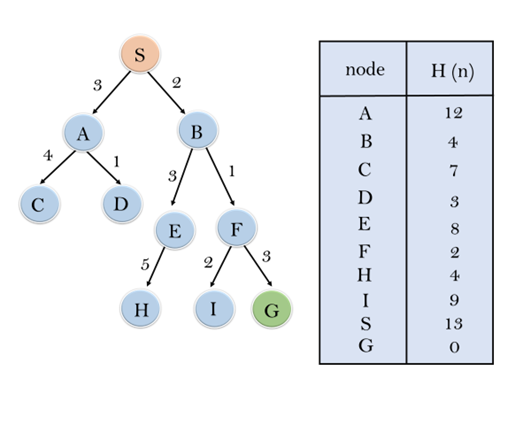
In this search example, we are using two lists which are OPEN and CLOSED Lists. Following are the iteration for traversing the above example.

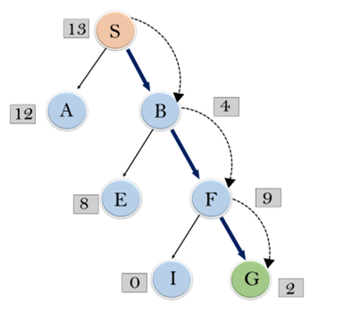
Expand the nodes of S and put in the CLOSED list

Initialization: Open [A, B], Closed [S]

Iteration 1: Open [A], Closed [S, B]

Iteration 2: Open [E, F, A], Closed [S, B]

: Open [E, A], Closed [S, B, F]

Iteration 3: Open [I, G, E, A], Closed [S, B, F]

: Open [I, E, A], Closed [S, B, F, G]

Hence the final solution path will be: S----> B----->F----> G

Time Complexity: The worst case time complexity of Greedy best first search is O(bm).

Space Complexity: The worst case space complexity of Greedy best first search is O(bm). Where, m is the maximum depth of the search space.

Complete: Greedy best-first search is also incomplete, even if the given state space is finite.

Optimal: Greedy best first search algorithm is not optimal.

Key takeaway

Greedy best-first search algorithm always selects the path which appears best at that moment. It is the combination of depth-first search and breadth-first search algorithms.

3.4 A* Search Algorithm

A* search is the most commonly known form of best-first search. It uses heuristic function h(n), and cost to reach the node n from the start state g(n). It has combined features of UCS and greedy best-first search, by which it solve the problem efficiently. A* search algorithm finds the shortest path through the search space using the heuristic function. This search algorithm expands less search tree and provides optimal result faster. A* algorithm is similar to UCS except that it uses g(n)+h(n) instead of g(n).

In A* search algorithm, we use search heuristic as well as the cost to reach the node. Hence we can combine both costs as following, and this sum is called as a fitness number.

At each point in the search space, only those node is expanded which have the lowest value of f(n), and the algorithm terminates when the goal node is found.

Algorithm of A* search:

Step1: Place the starting node in the OPEN list.

Step 2: Check if the OPEN list is empty or not, if the list is empty then return failure and stops.

Step 3: Select the node from the OPEN list which has the smallest value of evaluation function (g+h), if node n is goal node then return success and stop, otherwise

Step 4: Expand node n and generate all of its successors, and put n into the closed list. For each successor n', check whether n' is already in the OPEN or CLOSED list, if not then compute evaluation function for n' and place into Open list.

Step 5: Else if node n' is already in OPEN and CLOSED, then it should be attached to the back pointer which reflects the lowest g(n') value.

Step 6: Return to Step 2.

Advantages:

●        A* search algorithm is the best algorithm than other search algorithms.

●        A* search algorithm is optimal and complete.

●        This algorithm can solve very complex problems.

Disadvantages:

●        It does not always produce the shortest path as it mostly based on heuristics and approximation.

●        A* search algorithm has some complexity issues.

●        The main drawback of A* is memory requirement as it keeps all generated nodes in the memory, so it is not practical for various large-scale problems.

Example:

In this example, we will traverse the given graph using the A* algorithm. The heuristic value of all states is given in the below table so we will calculate the f(n) of each state using the formula f(n)= g(n) + h(n), where g(n) is the cost to reach any node from start state.

Here we will use OPEN and CLOSED list.

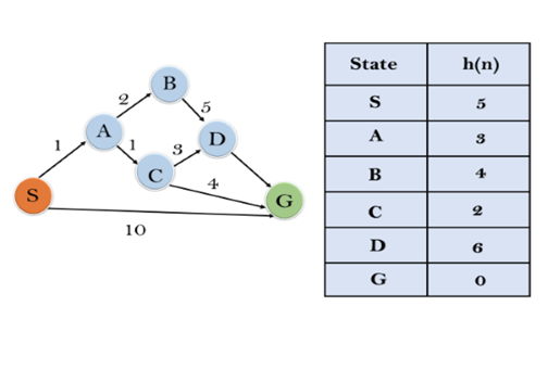
Solution:

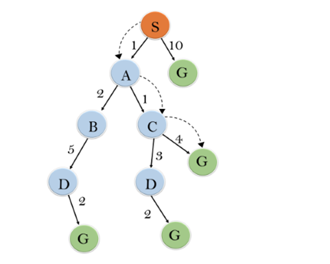
Initialization: {(S, 5)}

Iteration1: {(S--> A, 4), (S-->G, 10)}

Iteration2: {(S--> A-->C, 4), (S--> A-->B, 7), (S-->G, 10)}

Iteration3: {(S--> A-->C--->G, 6), (S--> A-->C--->D, 11), (S--> A-->B, 7), (S-->G, 10)}

Iteration 4 will give the final result, as S--->A--->C--->G it provides the optimal path with cost 6.

Points to remember:

●        A* algorithm returns the path which occurred first, and it does not search for all remaining paths.

●        The efficiency of A* algorithm depends on the quality of heuristic.

●        A* algorithm expands all nodes which satisfy the condition f(n) <="" li="">

Complete: A* algorithm is complete as long as:

●        Branching factor is finite.

●        Cost at every action is fixed.

Optimal: A* search algorithm is optimal if it follows below two conditions:

●        Admissible: the first condition requires for optimality is that h(n) should be an admissible heuristic for A* tree search. An admissible heuristic is optimistic in nature.

●        Consistency: Second required condition is consistency for only A* graph-search.

If the heuristic function is admissible, then A* tree search will always find the least cost path.

Time Complexity: The time complexity of A* search algorithm depends on heuristic function, and the number of nodes expanded is exponential to the depth of solution d. So the time complexity is O(b^d), where b is the branching factor.

Space Complexity: The space complexity of A* search algorithm is O(b^d).

Key takeaway

A* search is the most commonly known form of best-first search. It uses heuristic function h(n), and cost to reach the node n from the start state g(n). It has combined features of UCS and greedy best-first search, by which it solve the problem efficiently.

3.5 Hill Climbing

Hill Climbing Algorithm in Artificial Intelligence

●        Hill climbing algorithm is a local search algorithm which continuously moves in the direction of increasing elevation/value to find the peak of the mountain or best solution to the problem. It terminates when it reaches a peak value where no neighbor has a higher value.

●        Hill climbing algorithm is a technique which is used for optimizing the mathematical problems. One of the widely discussed examples of Hill climbing algorithm is Traveling-salesman Problem in which we need to minimize the distance traveled by the salesman.

●        It is also called greedy local search as it only looks to its good immediate neighbor state and not beyond that.

●        A node of hill climbing algorithm has two components which are state and value.

●        Hill Climbing is mostly used when a good heuristic is available.

●        In this algorithm, we don't need to maintain and handle the search tree or graph as it only keeps a single current state.

Features of Hill Climbing:

Following are some main features of Hill Climbing Algorithm:

●        Generate and Test variant: Hill Climbing is the variant of Generate and Test method. The Generate and Test method produce feedback which helps to decide which direction to move in the search space.

●        Greedy approach: Hill-climbing algorithm search moves in the direction which optimizes the cost.

●        No backtracking: It does not backtrack the search space, as it does not remember the previous states.

State-space Diagram for Hill Climbing:

The state-space landscape is a graphical representation of the hill-climbing algorithm which is showing a graph between various states of algorithm and Objective function/Cost.

On Y-axis we have taken the function which can be an objective function or cost function, and state-space on the x-axis. If the function on Y-axis is cost then, the goal of search is to find the global minimum and local minimum. If the function of Y-axis is Objective function, then the goal of the search is to find the global maximum and local maximum.

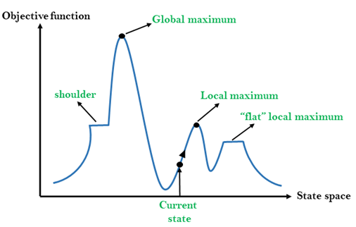
Different regions in the state space landscape:

Local Maximum: Local maximum is a state which is better than its neighbor states, but there is also another state which is higher than it.

Global Maximum: Global maximum is the best possible state of state space landscape. It has the highest value of objective function.

Current state: It is a state in a landscape diagram where an agent is currently present.

Flat local maximum: It is a flat space in the landscape where all the neighbor states of current states have the same value.

Shoulder: It is a plateau region which has an uphill edge.

Types of Hill Climbing Algorithm:

●        Simple hill Climbing:

●        Steepest-Ascent hill-climbing:

●        Stochastic hill Climbing:

1. Simple Hill Climbing:

Simple hill climbing is the simplest way to implement a hill climbing algorithm. It only evaluates the neighbor node state at a time and selects the first one which optimizes current cost and set it as a current state. It only checks it's one successor state, and if it finds better than the current state, then move else be in the same state. This algorithm has the following features:

●        Less time consuming

●        Less optimal solution and the solution is not guaranteed

Algorithm for Simple Hill Climbing:

●        Step 1: Evaluate the initial state, if it is goal state then return success and Stop.

●        Step 2: Loop Until a solution is found or there is no new operator left to apply.

●        Step 3: Select and apply an operator to the current state.

●        Step 4: Check new state:

1. If it is goal state, then return success and quit.
2. Else if it is better than the current state then assign new state as a current state.
3. Else if not better than the current state, then return to step2.

●        Step 5: Exit.

2. Steepest-Ascent hill climbing:

The steepest-Ascent algorithm is a variation of simple hill climbing algorithm. This algorithm examines all the neighboring nodes of the current state and selects one neighbor node which is closest to the goal state. This algorithm consumes more time as it searches for multiple neighbors

Algorithm for Steepest-Ascent hill climbing:

●        Step 1: Evaluate the initial state, if it is goal state then return success and stop, else make current state as initial state.

●        Step 2: Loop until a solution is found or the current state does not change.

1. Let SUCC be a state such that any successor of the current state will be better than it.
2. For each operator that applies to the current state:
   1. Apply the new operator and generate a new state.
   2. Evaluate the new state.
   3. If it is goal state, then return it and quit, else compare it to the SUCC.
   4. If it is better than SUCC, then set new state as SUCC.
   5. If the SUCC is better than the current state, then set current state to SUCC.

●        Step 5: Exit.

3. Stochastic hill climbing:

Stochastic hill climbing does not examine for all its neighbor before moving. Rather, this search algorithm selects one neighbor node at random and decides whether to choose it as a current state or examine another state.

Problems in Hill Climbing Algorithm:

1. Local Maximum: A local maximum is a peak state in the landscape which is better than each of its neighboring states, but there is another state also present which is higher than the local maximum.

Solution: Backtracking technique can be a solution of the local maximum in state space landscape. Create a list of the promising path so that the algorithm can backtrack the search space and explore other paths as well.

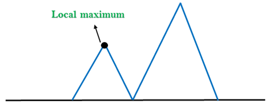
Fig 2: Local maximum

2. Plateau: A plateau is the flat area of the search space in which all the neighbor states of the current state contains the same value, because of this algorithm does not find any best direction to move. A hill-climbing search might be lost in the plateau area.

Solution: The solution for the plateau is to take big steps or very little steps while searching, to solve the problem. Randomly select a state which is far away from the current state so it is possible that the algorithm could find non-plateau region

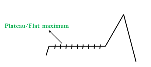
Fig 3: Plateau

3. Ridges: A ridge is a special form of the local maximum. It has an area which is higher than its surrounding areas, but itself has a slope, and cannot be reached in a single move.

Solution: With the use of bidirectional search, or by moving in different directions, we can improve this problem.

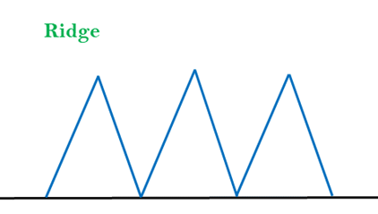
Fig 4: Ridge

Key takeaway

Hill climbing algorithm is a local search algorithm which continuously moves in the direction of increasing elevation/value to find the peak of the mountain or best solution to the problem. It terminates when it reaches a peak value where no neighbor has a higher value.

3.6 Simulated Annealing

A hill-climbing algorithm which never makes a move towards a lower value guaranteed to be incomplete because it can get stuck on a local maximum. And if algorithm applies a random walk, by moving a successor, then it may complete but not efficient. Simulated Annealing is an algorithm which yields both efficiency and completeness.

In mechanical term Annealing is a process of hardening a metal or glass to a high temperature then cooling gradually, so this allows the metal to reach a low-energy crystalline state. The same process is used in simulated annealing in which the algorithm picks a random move, instead of picking the best move. If the random move improves the state, then it follows the same path. Otherwise, the algorithm follows the path which has a probability of less than 1 or it moves downhill and chooses another path.

Problem: Given a cost function f: R^n –> R, find an n-tuple that minimizes the value of f. Note that minimizing the value of a function is algorithmically equivalent to maximization (since we can redefine the cost function as 1-f).

Many of you with a background in calculus/analysis are likely familiar with simple optimization for single variable functions. For instance, the function f(x) = x^2 + 2x can be optimized setting the first derivative equal to zero, obtaining the solution x = -1 yielding the minimum value f(-1) = -1. This technique suffices for simple functions with few variables. However, it is often the case that researchers are interested in optimizing functions of several variables, in which case the solution can only be obtained computationally.

One excellent example of a difficult optimization task is the chip floor planning problem. Imagine you’re working at Intel and you’re tasked with designing the layout for an integrated circuit. You have a set of modules of different shapes/sizes and a fixed area on which the modules can be placed. There are a number of objectives you want to achieve: maximizing ability for wires to connect components, minimize net area, minimize chip cost, etc. With these in mind, you create a cost function, taking all, say, 1000 variable configurations and returning a single real value representing the ‘cost’ of the input configuration. We call this the objective function, since the goal is to minimize its value.

A naive algorithm would be a complete space search — we search all possible configurations until we find the minimum. This may suffice for functions of few variables, but the problem we have in mind would entail such a brute force algorithm to fun in O(n!).

Due to the computational intractability of problems like these, and other NP-hard problems, many optimization heuristics have been developed in an attempt to yield a good, albeit potentially suboptimal, value. In our case, we don’t necessarily need to find a strictly optimal value — finding a near-optimal value would satisfy our goal. One widely used technique is simulated annealing, by which we introduce a degree of stochasticity, potentially shifting from a better solution to a worse one, in an attempt to escape local minima and converge to a value closer to the global optimum.

Simulated annealing is based on metallurgical practices by which a material is heated to a high temperature and cooled. At high temperatures, atoms may shift unpredictably, often eliminating impurities as the material cools into a pure crystal. This is replicated via the simulated annealing optimization algorithm, with energy state corresponding to current solution.

In this algorithm, we define an initial temperature, often set as 1, and a minimum temperature, on the order of 10^-4. The current temperature is multiplied by some fraction alpha and thus decreased until it reaches the minimum temperature. For each distinct temperature value, we run the core optimization routine a fixed number of times. The optimization routine consists of finding a neighboring solution and accepting it with probability e^(f(c) – f(n)) where c is the current solution and n is the neighboring solution.

A neighboring solution is found by applying a slight perturbation to the current solution. This randomness is useful to escape the common pitfall of optimization heuristics — getting trapped in local minima. By potentially accepting a less optimal solution than we currently have, and accepting it with probability inverse to the increase in cost, the algorithm is more likely to converge near the global optimum. Designing a neighbor function is quite tricky and must be done on a case by case basis, but below are some ideas for finding neighbors in locational optimization problems.

●        Move all points 0 or 1 units in a random direction

●        Shift input elements randomly

●        Swap random elements in input sequence

●        Permute input sequence

●        Partition input sequence into a random number of segments and permute segments

One caveat is that we need to provide an initial solution so the algorithm knows where to start. This can be done in two ways: (1) using prior knowledge about the problem to input a good starting point and (2) generating a random solution. Although generating a random solution is worse and can occasionally inhibit the success of the algorithm, it is the only option for problems where we know nothing about the landscape.

There are many other optimization techniques, although simulated annealing is a useful, stochastic optimization heuristic for large, discrete search spaces in which optimality is prioritized over time. Below, I’ve included a basic framework for locational-based simulated annealing (perhaps the most applicable flavor of optimization for simulated annealing). Of course, the cost function, candidate generation function, and neighbor function must be defined based on the specific problem at hand, although the core optimization routine has already been implemented.

Output:

-1.0

[X, -, X, X, X]

[-, X, X, X, X]

[-, X, X, X, X]

[-, X, X, X, X]

[-, X, X, X, X]

Key takeaway

In mechanical term Annealing is a process of hardening a metal or glass to a high temperature then cooling gradually, so this allows the metal to reach a low-energy crystalline state.

Simulated annealing is based on metallurgical practices by which a material is heated to a high temperature and cooled.

3.7 Genetic Algorithm

Genetic Algorithm (GA) is a search-based optimization technique based on the principles of Genetics and Natural Selection. It is frequently used to find optimal or near-optimal solutions to difficult problems which otherwise would take a lifetime to solve. It is frequently used to solve optimization problems, in research, and in machine learning.

Introduction to Optimization

Optimization is the process of making something better. In any process, we have a set of inputs and a set of outputs as shown in the following figure.

Fig 5: Process

Optimization refers to finding the values of inputs in such a way that we get the “best” output values. The definition of “best” varies from problem to problem, but in mathematical terms, it refers to maximizing or minimizing one or more objective functions, by varying the input parameters.

The set of all possible solutions or values which the inputs can take make up the search space. In this search space, lies a point or a set of points which gives the optimal solution. The aim of optimization is to find that point or set of points in the search space.

What are Genetic Algorithms?

Nature has always been a great source of inspiration to all mankind. Genetic Algorithms (GAs) are search based algorithms based on the concepts of natural selection and genetics. GAs are a subset of a much larger branch of computation known as Evolutionary Computation.

GAs were developed by John Holland and his students and colleagues at the University of Michigan, most notably David E. Goldberg and has since been tried on various optimization problems with a high degree of success.

In GAs, we have a pool or a population of possible solutions to the given problem. These solutions then undergo recombination and mutation (like in natural genetics), producing new children, and the process is repeated over various generations. Each individual (or candidate solution) is assigned a fitness value (based on its objective function value) and the fitter individuals are given a higher chance to mate and yield more “fitter” individuals. This is in line with the Darwinian Theory of “Survival of the Fittest”.

In this way we keep “evolving” better individuals or solutions over generations, till we reach a stopping criterion.

Genetic Algorithms are sufficiently randomized in nature, but they perform much better than random local search (in which we just try various random solutions, keeping track of the best so far), as they exploit historical information as well.

Advantages of GAs

GAs have various advantages which have made them immensely popular. These include −

●        Does not require any derivative information (which may not be available for many real-world problems).

●        Is faster and more efficient as compared to the traditional methods.

●        Has very good parallel capabilities.

●        Optimizes both continuous and discrete functions and also multi-objective problems.

●        Provides a list of “good” solutions and not just a single solution.

●        Always gets an answer to the problem, which gets better over the time.

●        Useful when the search space is very large and there are a large number of parameters involved.

Limitations of GAs

Like any technique, GAs also suffer from a few limitations. These include −

●        GAs are not suited for all problems, especially problems which are simple and for which derivative information is available.

●        Fitness value is calculated repeatedly which might be computationally expensive for some problems.

●        Being stochastic, there are no guarantees on the optimality or the quality of the solution.

●        If not implemented properly, the GA may not converge to the optimal solution.

GA – Motivation

Genetic Algorithms have the ability to deliver a “good-enough” solution “fast-enough”. This makes genetic algorithms attractive for use in solving optimization problems. The reasons why GAs are needed are as follows −

Solving Difficult Problems

In computer science, there is a large set of problems, which are NP-Hard. What this essentially means is that, even the most powerful computing systems take a very long time (even years!) to solve that problem. In such a scenario, GAs prove to be an efficient tool to provide usable near-optimal solutions in a short amount of time.

Failure of Gradient Based Methods

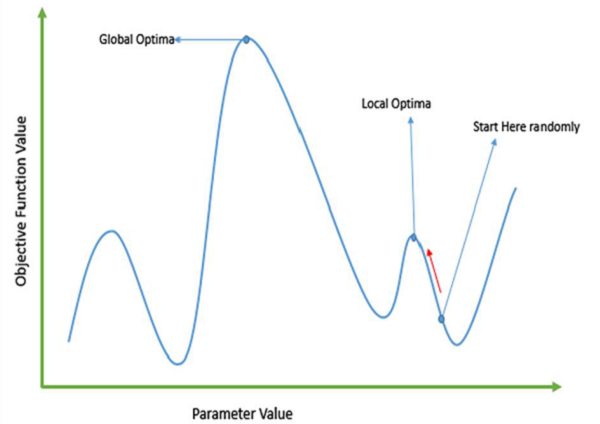
Traditional calculus based methods work by starting at a random point and by moving in the direction of the gradient, till we reach the top of the hill. This technique is efficient and works very well for single-peaked objective functions like the cost function in linear regression. But, in most real-world situations, we have a very complex problem called as landscapes, which are made of many peaks and many valleys, which causes such methods to fail, as they suffer from an inherent tendency of getting stuck at the local optima as shown in the following figure.

Getting a Good Solution Fast

Some difficult problems like the Travelling Salesperson Problem (TSP), have real-world applications like path finding and VLSI Design. Now imagine that you are using your GPS Navigation system, and it takes a few minutes (or even a few hours) to compute the “optimal” path from the source to destination. Delay in such real world applications is not acceptable and therefore a “good-enough” solution, which is delivered “fast” is what is required.

This section introduces the basic terminology required to understand GAs. Also, a generic structure of GAs is presented in both pseudo-code and graphical forms. The reader is advised to properly understand all the concepts introduced in this section and keep them in mind when reading other sections of this tutorial as well.

Basic Terminology

Before beginning a discussion on Genetic Algorithms, it is essential to be familiar with some basic terminology which will be used throughout this tutorial.

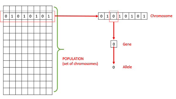
●        Population − It is a subset of all the possible (encoded) solutions to the given problem. The population for a GA is analogous to the population for human beings except that instead of human beings, we have Candidate Solutions representing human beings.

●        Chromosomes − A chromosome is one such solution to the given problem.

●        Gene − A gene is one element position of a chromosome.

●        Allele − It is the value a gene takes for a particular chromosome.

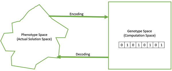
●        Genotype − Genotype is the population in the computation space. In the computation space, the solutions are represented in a way which can be easily understood and manipulated using a computing system.

●        Phenotype − Phenotype is the population in the actual real world solution space in which solutions are represented in a way they are represented in real world situations.

●        Decoding and Encoding − For simple problems, the phenotype and genotype spaces are the same. However, in most of the cases, the phenotype and genotype spaces are different. Decoding is a process of transforming a solution from the genotype to the phenotype space, while encoding is a process of transforming from the phenotype to genotype space. Decoding should be fast as it is carried out repeatedly in a GA during the fitness value calculation.

For example, consider the 0/1 Knapsack Problem. The Phenotype space consists of solutions which just contain the item numbers of the items to be picked.

However, in the genotype space it can be represented as a binary string of length n (where n is the number of items). A 0 at position x represents that xth item is picked while a 1 represents the reverse. This is a case where genotype and phenotype spaces are different.

●        Fitness Function − A fitness function simply defined is a function which takes the solution as input and produces the suitability of the solution as the output. In some cases, the fitness function and the objective function may be the same, while in others it might be different based on the problem.

●        Genetic Operators − These alter the genetic composition of the offspring. These include crossover, mutation, selection, etc.

Basic Structure

The basic structure of a GA is as follows −

We start with an initial population (which may be generated at random or seeded by other heuristics), select parents from this population for mating. Apply crossover and mutation operators on the parents to generate new off-springs. And finally these off-springs replace the existing individuals in the population and the process repeats. In this way genetic algorithms actually try to mimic the human evolution to some extent.

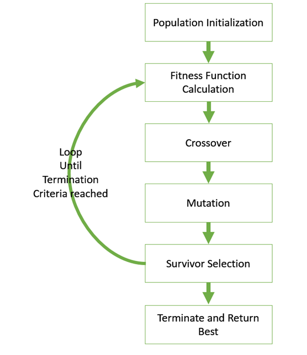
A generalized pseudo-code for a GA is explained in the following program −

GA()

Initialize population

Find fitness of population

While (termination criteria is reached) do

Parent selection

Crossover with probability pc

Mutation with probability pm

Decode and fitness calculation

Survivor selection

Find best

Return best

Key takeaway

Genetic Algorithm (GA) is a search-based optimization technique based on the principles of Genetics and Natural Selection.

GAs were developed by John Holland and his students and colleagues at the University of Michigan, most notably David E. Goldberg and has since been tried on various optimization problems with a high degree of success.

3.8 Constraint Satisfaction Problems

Constraint satisfaction problems (CSPs) are mathematical problems in which the state of a group of objects must meet a set of constraints or limitations. Constraint satisfaction methods are used to solve CSPs, which express the entities in a problem as a homogeneous set of finite constraints over variables. CSPs are the focus of research in both artificial intelligence and operations research, because the regularity of their formulation provides a common framework for analysing and solving issues from a wide range of seemingly unrelated families. CSPs are frequently complex, necessitating the use of a combination of heuristics and combinatorial search methods to solve in a reasonable amount of time. Constraint programming (CP) is a branch of computer science that specialises in solving difficulties like these.

A constraint satisfaction problem (CSP) consists of

●        A set of variables,

●        A domain for each variable, and

●        A set of constraints.

The aim is to choose a value for each variable so that the resulting possible world satisfies the constraints; we want a model of the constraints.

A finite CSP has a finite set of variables and a finite domain for each variable. Many of the methods considered in this chapter only work for finite CSPs, although some are designed for infinite, even continuous, domains.

The multidimensional aspect of these problems, where each variable can be seen as a separate dimension, makes them difficult to solve but also provides structure that can be exploited.

Given a CSP, there are a number of tasks that can be performed:

●        Determine whether or not there is a model.

●        Find a model.

●        Find all of the models or enumerate the models.

●        Count the number of models.

●        Find the best model, given a measure of how good models are.

●        Determine whether some statement holds in all models.

Some of the methods can also determine if there is no solution. What may be more surprising is that some of the methods can find a model if one exists, but they cannot tell us that there is no model if none exists.

CSPs are very common, so it is worth trying to find relatively efficient ways to solve them. Determining whether there is a model for a CSP with finite domains is NP-hard and no known algorithms exist to solve such problems that do not use exponential time in the worst case. However, just because a problem is NP-hard does not mean that all instances are difficult to solve. Many instances have structure that can be exploited.

Key takeaway

Constraint satisfaction problems (CSPs) are mathematical problems in which the state of a group of objects must meet a set of constraints or limitations. Constraint satisfaction methods are used to solve CSPs, which express the entities in a problem as a homogeneous set of finite constraints over variables.

3.9 Adversarial Search

Adversarial search is a game-playing technique where the agents are surrounded by a competitive environment. A conflicting goal is given to the agents (multiagent).

These agents compete with one another and try to defeat one another in order to win the game.

Such conflicting goals give rise to the adversarial search. Here, game-playing means discussing those games where human intelligence and logic factor is used, excluding other factors such as luck factor. Tic-tac-toe, chess, checkers, etc., are such type of games where no luck factor works, only mind works.

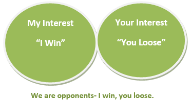
Mathematically, this search is based on the concept of ‘Game Theory.’ According to game theory, a game is played between two players. To complete the game, one has to win the game and the other looses automatically.’

Techniques required to get the best optimal solution

There is always a need to choose those algorithms which provide the best optimal solution in a limited time. So, we use the following techniques which could fulfill our requirements:

Elements of Game Playing search

To play a game, we use a game tree to know all the possible choices and to pick the best one out. There are following elements of a game-playing:

For example, in chess, tic-tac-toe, we have two or three possible outcomes. Either to win, to lose, or to draw the match with values +1, -1 or 0.

Let’s understand the working of the elements with the help of a game tree designed for tic-tac-toe. Here, the node represents the game state and edges represent the moves taken by the players.

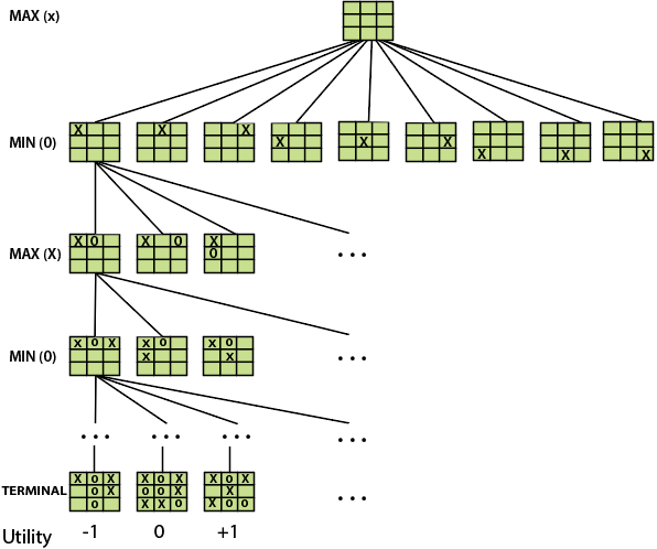
A game-tree for tic-tac-toe

Types of algorithms in Adversarial search

In a normal search, we follow a sequence of actions to reach the goal or to finish the game optimally. But in an adversarial search, the result depends on the players which will decide the result of the game. It is also obvious that the solution for the goal state will be an optimal solution because the player will try to win the game with the shortest path and under limited time.

There are following types of adversarial search:

Key takeaway

Adversarial search is a game-playing technique where the agents are surrounded by a competitive environment. A conflicting goal is given to the agents (multiagent).

3.10 Games

Adversarial search is a sort of search that examines the problem that arises when we attempt to plan ahead of the world while other agents plan against us.

●      In previous topics, we looked at search strategies that are purely associated with a single agent attempting to find a solution, which is often stated as a series of activities.

●      However, in game play, there may be moments when more than one agent is looking for the same answer in the same search field.

●      A multi-agent environment is one in which there are multiple agents, each of which is an opponent to the others and competes against them. Each agent must think about what another agent is doing and how that activity affects their own performance.

●      Adversarial searches, also referred to as Games, are searches in which two or more players with conflicting goals try to find a solution in the same search space.

●      The two fundamental variables that contribute in the modeling and solving of games in AI are a Search problem and a heuristic evaluation function.

Types of Games in AI

●      Perfect information: A game with perfect information is one in which agents have complete visibility of the board. Agents can see each other's movements and have access to all game information. Examples include chess, checkers, go, and other games.

●      Imperfect information: Tic-tac-toe, Battleship, blind, Bridge, and other games with incomplete information are known as such because the agents do not have all of the information and are unaware of what is going on.

●      Deterministic games: Deterministic games have no element of chance and follow a strict pattern and set of rules. Examples include chess, checkers, go, tic-tac-toe, and other games.

●       Non-deterministic games: Non-deterministic games are those with a number of unpredictable events and a chance or luck aspect. Dice or cards are used to introduce the element of chance or luck. These are unpredictably generated, and each action reaction is unique. Stochastic games are another name for these types of games.

Example: Backgammon, Monopoly, Poker, etc.

Search for games

Searches in which two or more players with conflicting goals are trying to explore the same search space for the solution, are called adversarial searches, often known as Games.

Games are modeled as a Search problem and heuristic evaluation function, and these are the two main factors which help to model and solve games in AI.

Types of Games in AI:

• Perfect information: A game with the perfect information is that in which agents can look into the complete board. Agents have all the information about the game, and they can see each other moves also. Examples are Chess, Checkers, Go, etc.
• Imperfect information: If in a game agent do not have all information about the game and not aware with what's going on, such type of games are called the game with imperfect information, such as tic-tac-toe, Battleship, blind, Bridge, etc.
• Deterministic games: Deterministic games are those games which follow a strict pattern and set of rules for the games, and there is no randomness associated with them. Examples are chess, Checkers, Go, tic-tac-toe, etc.
• Non-deterministic games: Non-deterministic are those games which have various unpredictable events and has a factor of chance or luck. This factor of chance or luck is introduced by either dice or cards. These are random, and each action response is not fixed. Such games are also called as stochastic games.

Example: Backgammon, Monopoly, Poker, etc.

Zero-Sum Game

• Zero-sum games are adversarial search which involves pure competition.
• In Zero-sum game each agent's gain or loss of utility is exactly balanced by the losses or gains of utility of another agent.
• One player of the game try to maximize one single value, while other player tries to minimize it.
• Each move by one player in the game is called as ply.
• Chess and tic-tac-toe are examples of a Zero-sum game.

Zero-sum game: Embedded thinking

The Zero-sum game involved embedded thinking in which one agent or player is trying to figure out:

• What to do.
• How to decide the move
• Needs to think about his opponent as well
• The opponent also thinks what to do

Each of the players is trying to find out the response of his opponent to their actions. This requires embedded thinking or backward reasoning to solve the game problems in AI.

Formalization of the problem:

A game can be defined as a type of search in AI which can be formalized of the following elements:

• Initial state: It specifies how the game is set up at the start.
• Player(s): It specifies which player has moved in the state space.
• Action(s): It returns the set of legal moves in state space.
• Result(s, a): It is the transition model, which specifies the result of moves in the state space.
• Terminal-Test(s): Terminal test is true if the game is over, else it is false at any case. The state where the game ends is called terminal states.
• Utility(s, p): A utility function gives the final numeric value for a game that ends in terminal states s for player p. It is also called payoff function. For Chess, the outcomes are a win, loss, or draw and its payoff values are +1, 0, ½. And for tic-tac-toe, utility values are +1, -1, and 0.

Key takeaway

Adversarial search is a type of search in which we look at the issue that develops when we try to plan ahead of the world while other agents plan against us.

Games are modeled as a Search problem and a heuristic evaluation function, which are the two primary variables that aid in the modeling and solving of games in AI.
 

3.11 Optimal decisions and strategies in games

A sequence of actions leading to a goal state—a terminal state that is a win—would be the best solution in a typical search problem. MIN has something to say regarding STRATEGY in adversarial search. As a result, MAX must devise a contingent strategy that defines MAX's initial move, then MAX's moves in the states resulting from every potential MIN reaction, then MAX's moves in the states resulting from every possible MIN response to those moves, and so forth. This is exactly the same as the AND–OR search method (Fig), with MAX acting as OR and MIN acting as AND. When playing an infallible opponent, an optimal strategy produces results that are as least as excellent as any other plan. We'll start by demonstrating how to find the best plan.

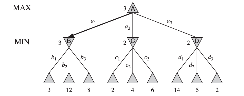
Fig 6: A two-ply game tree

The △ nodes are “MAX nodes,” in which it is MAX’s turn to move, and the  nodes are ▽ “MIN nodes.” The terminal nodes show the utility values for MAX; the other nodes are labeled with their minimax values. MAX’s best move at the root is a1, because it leads to the state with the highest minimax value, and MIN’s best reply is b1, because it leads to the state with the lowest minimax value.

We'll move to the trivial game in Figure  since even a simple game like tic-tac-toe is too complex for us to draw the full game tree on one page. MAX's root node moves are designated by the letters a1, a2, and a3. MIN's probable answers to a1 are b1, b2, b3, and so on. This game is over after MAX and MIN each make one move. (In game terms, this tree is one move deep and consists of two half-moves, each of which PLY is referred to as a ply). The terminal states in this game have utility values ranging from 2 to 14.

The optimal strategy can be found from the minimax value of each node, which we express as MINIMAX, given a game tree (n). The utility (for MAX) of being in the corresponding state is the node's minimax value, assuming that both players play optimally from there through the finish of the game. The usefulness of a terminal state is obviously its minimax value. Furthermore, if given the option, MAX prefers to shift to a maximum value state, whereas MIN wants to move to a minimum value state. So here's what we've got:

Let's put these definitions to work on the game tree shown in Fig. The UTILITY function in the game provides utility values to the terminal nodes on the bottom level. Because the first MIN node, B, has three successor states with the values 3, 12, and 8, its minimax value is 3. The other two MIN nodes have the same minimax value of 2. The root node is a MAX node, with minimax values of 3, 2, and 2 for its successor states, giving it a minimax value of 3. We can also find the root of the minimax decision: action a1 is the best choice for MAX since it leads to the highest minimax value state.

This concept of optimal MAX play requires that MIN plays optimally as well, maximising MAX's worst-case outcome. What if MIN's performance isn't up to par? Then it's a simple matter of demonstrating that MAX will perform even better. Other methods may perform better against suboptimal opponents than the minimax strategy, but they must perform worse against ideal opponents.

Key takeaway

A sequence of actions leading to a goal state—a terminal state that is a win—would be the best solution in a typical search problem. MIN has something to say regarding STRATEGY in adversarial search.

3.12 Minimax search

In artificial intelligence, minimax is a decision-making strategy under game theory, which is used to minimize the losing chances in a game and to maximize the winning chances. This strategy is also known as ‘Minmax,’ ’MM,’ or ‘Saddle point.’ Basically, it is a two-player game strategy where if one wins, the other loose the game. This strategy simulates those games that we play in our day-to-day life. Like, if two persons are playing chess, the result will be in favour of one player and will unfavoured the other one. The person who will make his best try, efforts as well as cleverness, will surely win.

We can easily understand this strategy via game tree– where the nodes represent the states of the game and edges represent the moves made by the players in the game.

Players will be two namely:

They both play the game alternatively, i.e., turn by turn and following the above strategy, i.e., if one wins, the other will definitely lose it. Both players look at one another as competitors and will try to defeat one-another, giving their best.

In minimax strategy, the result of the game or the utility value is generated by a heuristic function by propagating from the initial node to the root node. It follows the backtracking technique and backtracks to find the best choice. MAX will choose that path which will increase its utility value and MIN will choose the opposite path which could help it to minimize MAX’s utility value.

MINIMAX Algorithm

MINIMAX algorithm is a backtracking algorithm where it backtracks to pick the best move out of several choices. MINIMAX strategy follows the DFS (Depth-first search) concept. Here, we have two players MIN and MAX, and the game is played alternatively between them, i.e., when MAX made a move, then the next turn is of MIN. It means the move made by MAX is fixed and, he cannot change it. The same concept is followed in DFS strategy, i.e., we follow the same path and cannot change in the middle. That’s why in MINIMAX algorithm, instead of BFS, we follow DFS.

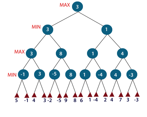
Fig 7: Min Max

For example, in the above figure, the two players MAX and MIN are there. MAX starts the game by choosing one path and propagating all the nodes of that path. Now, MAX will backtrack to the initial node and choose the best path where his utility value will be the maximum. After this, its MIN chance. MIN will also propagate through a path and again will backtrack, but MIN will choose the path which could minimize MAX winning chances or the utility value.

So, if the level is minimizing, the node will accept the minimum value from the successor nodes. If the level is maximizing, the node will accept the maximum value from the successor.

Pseudo-code for MinMax Algorithm:

Function minimax(node, depth, maximizingPlayer) is 

If depth ==0 or node is a terminal node then 

Return static evaluation of node 

If MaximizingPlayer then      // for Maximizer Player 

MaxEva= -infinity           

For each child of node do 

Eva= minimax(child, depth-1, false) 

MaxEva= max(maxEva,eva)        //gives Maximum of the values 

Return maxEva 

Else                         // for Minimizer player 

MinEva= +infinity  

For each child of node do 

Eva= minimax(child, depth-1, true) 

MinEva= min(minEva, eva)         //gives minimum of the values 

Return minEva 

Initial call:

Minimax(node, 3, true)

Properties

●      Complete - The Min-Max algorithm has reached its conclusion. In the finite search tree, it will undoubtedly locate a solution (if one exists).

●      If both opponents are playing optimally, the Min-Max algorithm is optimal.

●      Time complexity - Because the Min-Max method executes DFS for the game-tree, its time complexity is O(bm), where b is the game-branching tree's factor and m is the tree's maximum depth.

●      Space Complexity - The Mini-max method has a space complexity of O, which is identical to DFS (bm).

Limitations

The biggest disadvantage of the minimax algorithm is that it becomes extremely slow while playing complex games like chess or go. This style of game contains a lot of branching, and the player has a lot of options to choose from. The alpha-beta pruning technique can help to overcome this constraint of the minimax algorithm.

Key takeaway

In artificial intelligence, minimax is a decision-making strategy under game theory, which is used to minimize the losing chances in a game and to maximize the winning chances. This strategy is also known as ‘Minmax,’ ’MM,’ or ‘Saddle point.’ Basically, it is a two-player game strategy where if one wins, the other loose the game.

3.13 Alpha - Beta pruning

●        Alpha-beta pruning is a modified version of the minimax algorithm. It is an optimization technique for the minimax algorithm.

●        As we have seen in the minimax search algorithm that the number of game states it has to examine are exponential in depth of the tree. Since we cannot eliminate the exponent, but we can cut it to half. Hence there is a technique by which without checking each node of the game tree we can compute the correct minimax decision, and this technique is called pruning. This involves two threshold parameter Alpha and beta for future expansion, so it is called alpha-beta pruning. It is also called as Alpha-Beta Algorithm.

●        Alpha-beta pruning can be applied at any depth of a tree, and sometimes it not only prune the tree leaves but also entire sub-tree.

●        The two-parameter can be defined as:

1. Alpha: The best (highest-value) choice we have found so far at any point along the path of Maximizer. The initial value of alpha is -∞.
2. Beta: The best (lowest-value) choice we have found so far at any point along the path of Minimizer. The initial value of beta is +∞.

●        The Alpha-beta pruning to a standard minimax algorithm returns the same move as the standard algorithm does, but it removes all the nodes which are not really affecting the final decision but making algorithm slow. Hence by pruning these nodes, it makes the algorithm fast.

Note: To better understand this topic, kindly study the minimax algorithm.

Condition for Alpha-beta pruning:

The main condition which required for alpha-beta pruning is:

α>=β  

Pseudo-code for Alpha-beta Pruning:

1. Function minimax(node, depth, alpha, beta, maximizingPlayer) is  
2. If depth ==0 or node is a terminal node then  
3. Return static evaluation of node  
4.  
5. If MaximizingPlayer then      // for Maximizer Player  
6.   MaxEva= -infinity            
7.   For each child of node do  
8.   Eva= minimax(child, depth-1, alpha, beta, False)  
9.  MaxEva= max(maxEva, eva)   
10.  Alpha= max(alpha, maxEva)      
11.   If beta<=alpha  
12. Break  
13. Return maxEva  
14.    
15. Else                         // for Minimizer player  
16.   MinEva= +infinity   
17.   For each child of node do  
18.   Eva= minimax(child, depth-1, alpha, beta, true)  
19.   MinEva= min(minEva, eva)   
20.   Beta= min(beta, eva)  
21.    If beta<=alpha  
22.  Break          
23. Return minEva  

Working of Alpha-Beta Pruning:

Let's take an example of two-player search tree to understand the working of Alpha-beta pruning

Step 1: At the first step the, Max player will start first move from node A where α= -∞ and β= +∞, these value of alpha and beta passed down to node B where again α= -∞ and β= +∞, and Node B passes the same value to its child D.

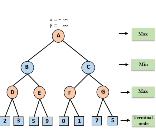
Step 2: At Node D, the value of α will be calculated as its turn for Max. The value of α is compared with firstly 2 and then 3, and the max (2, 3) = 3 will be the value of α at node D and node value will also 3.

Step 3: Now algorithm backtrack to node B, where the value of β will change as this is a turn of Min, Now β= +∞, will compare with the available subsequent nodes value, i.e. min (∞, 3) = 3, hence at node B now α= -∞, and β= 3.

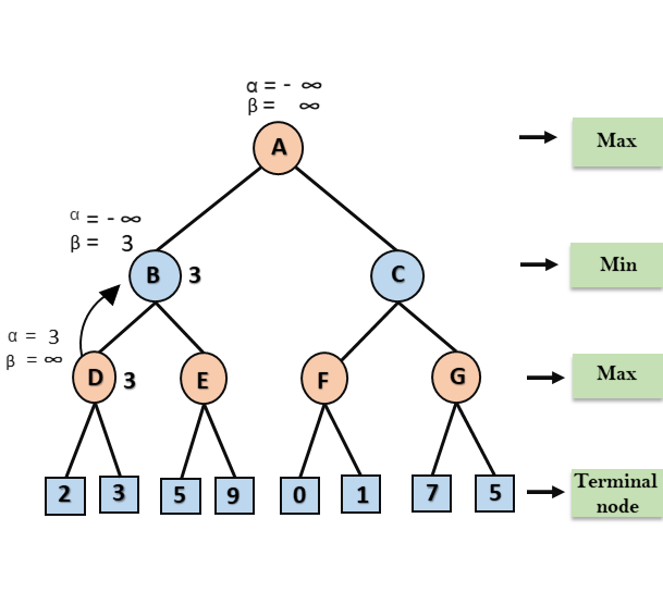
In the next step, algorithm traverse the next successor of Node B which is node E, and the values of α= -∞, and β= 3 will also be passed.

Step 4: At node E, Max will take its turn, and the value of alpha will change. The current value of alpha will be compared with 5, so max (-∞, 5) = 5, hence at node E α= 5 and β= 3, where α>=β, so the right successor of E will be pruned, and algorithm will not traverse it, and the value at node E will be 5.

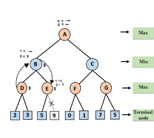
Step 5: At next step, algorithm again backtrack the tree, from node B to node A. At node A, the value of alpha will be changed the maximum available value is 3 as max (-∞, 3)= 3, and β= +∞, these two values now passes to right successor of A which is Node C.

At node C, α=3 and β= +∞, and the same values will be passed on to node F.

Step 6: At node F, again the value of α will be compared with left child which is 0, and max(3,0)= 3, and then compared with right child which is 1, and max(3,1)= 3 still α remains 3, but the node value of F will become 1.

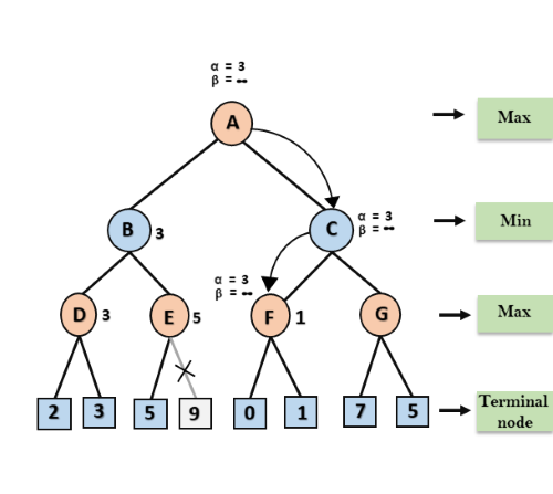
Step 7: Node F returns the node value 1 to node C, at C α= 3 and β= +∞, here the value of beta will be changed, it will compare with 1 so min (∞, 1) = 1. Now at C, α=3 and β= 1, and again it satisfies the condition α>=β, so the next child of C which is G will be pruned, and the algorithm will not compute the entire sub-tree G.

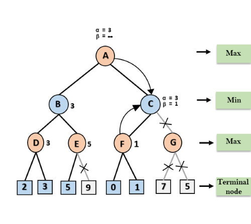
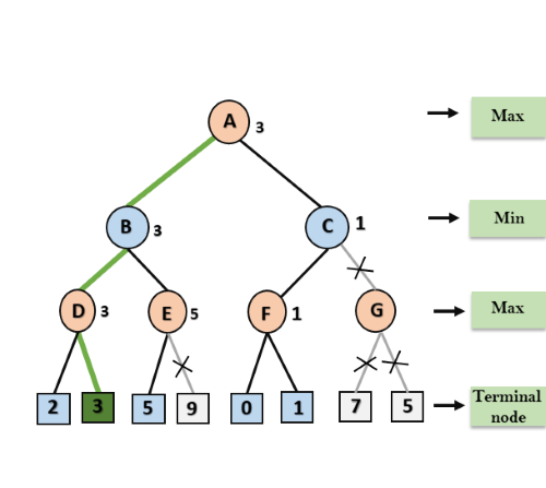
Step 8: C now returns the value of 1 to A here the best value for A is max (3, 1) = 3. Following is the final game tree which is the showing the nodes which are computed and nodes which has never computed. Hence the optimal value for the maximizer is 3 for this example.

Move Ordering in Alpha-Beta pruning:

The effectiveness of alpha-beta pruning is highly dependent on the order in which each node is examined. Move order is an important aspect of alpha-beta pruning.

It can be of two types:

●        Worst ordering: In some cases, alpha-beta pruning algorithm does not prune any of the leaves of the tree, and works exactly as minimax algorithm. In this case, it also consumes more time because of alpha-beta factors, such a move of pruning is called worst ordering. In this case, the best move occurs on the right side of the tree. The time complexity for such an order is O(bm).

●        Ideal ordering: The ideal ordering for alpha-beta pruning occurs when lots of pruning happens in the tree, and best moves occur at the left side of the tree. We apply DFS hence it first search left of the tree and go deep twice as minimax algorithm in the same amount of time. Complexity in ideal ordering is O(bm/2).

Rules to find good ordering:

Following are some rules to find good ordering in alpha-beta pruning:

●        Occur the best move from the shallowest node.

●        Order the nodes in the tree such that the best nodes are checked first.

●        Use domain knowledge while finding the best move. Ex: for Chess, try order: captures first, then threats, then forward moves, backward moves.

●        We can bookkeep the states, as there is a possibility that states may repeat.

Key points about alpha-beta pruning:

●        The Max player will only update the value of alpha.

●        The Min player will only update the value of beta.

●        While backtracking the tree, the node values will be passed to upper nodes instead of values of alpha and beta.

●        We will only pass the alpha, beta values to the child nodes.

3.14 Symbolic Logic: Syntax and semantics for propositional logic

Propositional logic (PL) is the simplest form of logic where all the statements are made by propositions. A proposition is a declarative statement which is either true or false. It is a technique of knowledge representation in logical and mathematical form.

Example:

1. a) It is Sunday.  
2. b) The Sun rises from West (False proposition)  
3. c) 3+3= 7(False proposition)  
4. d) 5 is a prime number.   

Following are some basic facts about propositional logic:

●        Propositional logic is also called Boolean logic as it works on 0 and 1.

●        In propositional logic, we use symbolic variables to represent the logic, and we can use any symbol for a representing a proposition, such A, B, C, P, Q, R, etc.

●        Propositions can be either true or false, but it cannot be both.

●        Propositional logic consists of an object, relations or function, and logical connectives.

●        These connectives are also called logical operators.

●        The propositions and connectives are the basic elements of the propositional logic.

●        Connectives can be said as a logical operator which connects two sentences.

●        A proposition formula which is always true is called tautology, and it is also called a valid sentence.

●        A proposition formula which is always false is called Contradiction.

●        A proposition formula which has both true and false values is called

●        Statements which are questions, commands, or opinions are not propositions such as "Where is Rohini", "How are you", "What is your name", are not propositions.

Syntax of propositional logic:

The syntax of propositional logic defines the allowable sentences for the knowledge representation. There are two types of Propositions:

1. Atomic Propositions
2. Compound propositions

●        Atomic Proposition: Atomic propositions are the simple propositions. It consists of a single proposition symbol. These are the sentences which must be either true or false.

Example:

1. a) 2+2 is 4, it is an atomic proposition as it is a true fact.  
2. b) "The Sun is cold" is also a proposition as it is a false fact.   

●        Compound proposition: Compound propositions are constructed by combining simpler or atomic propositions, using parenthesis and logical connectives.

Example:

1. a) "It is raining today, and street is wet."  
2. b) "Ankit is a doctor, and his clinic is in Mumbai."   

Logical Connectives:

Logical connectives are used to connect two simpler propositions or representing a sentence logically. We can create compound propositions with the help of logical connectives. There are mainly five connectives, which are given as follows:

1. Negation: A sentence such as ¬ P is called negation of P. A literal can be either Positive literal or negative literal.
2. Conjunction: A sentence which has ∧ connective such as, P ∧ Q is called a conjunction.
   Example: Rohan is intelligent and hardworking. It can be written as,
   P= Rohan is intelligent,
   Q= Rohan is hardworking. → P∧ Q.
3. Disjunction: A sentence which has ∨ connective, such as P ∨ Q. Is called disjunction, where P and Q are the propositions.
   Example: "Ritika is a doctor or Engineer",
   Here P= Ritika is Doctor. Q= Ritika is Doctor, so we can write it as P ∨ Q.
4. Implication: A sentence such as P → Q, is called an implication. Implications are also known as if-then rules. It can be represented as
   If it is raining, then the street is wet.

Let P= It is raining, and Q= Street is wet, so it is represented as P → Q

5.     Biconditional: A sentence such as P⇔ Q is a Biconditional sentence, example If I am breathing, then I am alive  P= I am breathing, Q= I am alive, it can be represented as P ⇔ Q.

Connective symbols	Word	Technical term	Example
	AND	Conjunction
∨	OR	Disjunction	A∨B
	Implies	Implication
⟺	If and only if	Biconditional	A⟺B
Or	Not	Negation	Aor

Truth Table:

In propositional logic, we need to know the truth values of propositions in all possible scenarios. We can combine all the possible combination with logical connectives, and the representation of these combinations in a tabular format is called Truth table. Following are the truth table for all logical connectives:

For negation

True	False
False	True

For conjunction

True	True	True
True	False	False
False	True	False
False	False	False

For disjunction

True	True	True
False	True	True
True	False	True
False	False	False

For implication

P	Q
True	True	True
True	False	False
False	True	True
False	False	True

For Biconditional

Truth table with three propositions:

We can build a proposition composing three propositions P, Q, and R. This truth table is made-up of 8n Tuples as we have taken three proposition symbols.

P	Q	R
True	True	True	False	True	False
True	True	False	True	True	True
True	False	True	False	True	False
True	False	False	True	True	True
False	True	True	False	True	False
False	True	False	True	True	True
False	False	True	False	False	True
False	False	False	True	False	True

Precedence of connectives:

Just like arithmetic operators, there is a precedence order for propositional connectors or logical operators. This order should be followed while evaluating a propositional problem. Following is the list of the precedence order for operators:

Note: For better understanding use parenthesis to make sure of the correct interpretations. Such as ¬R∨ Q, It can be interpreted as (¬R) ∨ Q.

Logical equivalence:

Logical equivalence is one of the features of propositional logic. Two propositions are said to be logically equivalent if and only if the columns in the truth table are identical to each other.

Let's take two propositions A and B, so for logical equivalence, we can write it as A⇔B. In below truth table we can see that column for ¬A∨ B and A→B, are identical hence A is Equivalent to B

A	B
T	T	F	T	T
T	F	F	F	F
F	T	T	T	T
F	F	T	T	T

Properties of Operators:

Commutativity:

• P∧ Q= Q ∧ P, or
• P ∨ Q = Q ∨ P.

Associativity:

• (P ∧ Q) ∧ R= P ∧ (Q ∧ R),
• (P ∨ Q) ∨ R= P ∨ (Q ∨ R)

Identity element:

• P ∧ True = P,
• P ∨ True= True.

Distributive:

• P∧ (Q ∨ R) = (P ∧ Q) ∨ (P ∧ R).
• P ∨ (Q ∧ R) = (P ∨ Q) ∧ (P ∨ R).

DE Morgan's Law:

• ¬ (P ∧ Q) = (¬P) ∨ (¬Q)
• ¬ (P ∨ Q) = (¬ P) ∧ (¬Q).

Double-negation elimination:

• ¬ (¬P) = P.

Limitations of Propositional logic:

●        We cannot represent relations like ALL, some, or none with propositional logic. Example:

All the girls are intelligent.

Some apples are sweet.

●        Propositional logic has limited expressive power.

●        In propositional logic, we cannot describe statements in terms of their properties or logical relationships.

Key takeaway

Propositional logic (PL) is the simplest form of logic where all the statements are made by propositions. A proposition is a declarative statement which is either true or false. It is a technique of knowledge representation in logical and mathematical form.

3.15 Syntax and semantics of FOPL

●      First-order logic is a type of knowledge representation used in artificial intelligence. It's a propositional logic variation.

●      FOL is expressive enough to convey natural language statements in a concise manner.

●      First-order logic is sometimes known as predicate logic or first-order predicate logic. First-order logic is a complex language for constructing information about objects and expressing relationships between them.

●      First-order logic (as does natural language) assumes not just that the world contains facts, as propositional logic does, but also that the world has the following:

○      Objects: People, numbers, colors, conflicts, theories, squares, pits, wumpus,

○      Relation: It can be a unary relation like red, round, or nearby, or an n-any relation like sister of, brother of, has color, or comes between.

○      Functions: Father of, best friend, third inning of, last inning of......

●      First-order logic contains two basic pieces as a natural language:

○      Syntax

○      Semantics

Syntax

Syntax has to do with what ‘things’ (symbols, notations) one is allowed to use in the language and in what way; there is/are a(n):

●       Alphabet

●       Language constructs

●       Sentences to assert knowledge

Logical connectives (⇒, ∧, ∨, and ⇐⇒), negation (¬), and parentheses. These will be used to recursively build complex formulas, just as was done for propositional logic.

Constants symbols are strings that will be interpreted as representing objects, e.g., Bob might be a constant.

Variable symbols will be used as “place holders” for quantifying over objects.

Predicate symbols Each has an arity (number of arguments) associated with it, which can be zero or some other finite value. Predicates will be used to represent object characteristics and relationships.

Zero-arity Because predicate symbols are viewed as propositions in first-order logic, propositional logic is subsumed. These assertions can be thought of as world properties.

Predicates with a single parameter can be thought of as specifying object attributes. If Rich is a single-arity predicate, then Rich (Bob) is used to indicate that Bob is wealthy. Multi-arity predicates are used to describe relationships between items.

Formula    Primitive Formula

| (Formula Connective Formula)

|  Sentence

| Qualifier Variable Formula

Primitive Formula  Predicate(Term,…,Term)

Term    Function(Term,…,Term)

| Constant

| Variable

Connectifier   

Quantifier  

Constant   any string that is not used as a variable predicate or function

Variable   any string that is not used as a constant predicate or function

Predicate   any string that is not used as a constant variable or function

Function   any string that is not used as a constant predicate or constant

Function symbols Each has a specific arity (number of input arguments) and is understood as a function that maps the stated number of input objects to objects. Allowing FatherOf to be a single-arity function symbol, the natural interpretation of FatherOf (Bob) is Bob's father.

Zero-arity function symbols are considered to be constants.

Universal and existential quantifier symbols will be used to quantify over objects. For example, ∀ x Alive(x) ⇒ Breathing(x) is a universally quantified statement that uses the variable x as a placeholder.

Semantics of First-Order Logic

As with all logics, the first step in determining the semantics of first-order logic is to define the models of first-order logic. Remember that one of the benefits of using first-order logic is that it allows us to freely discuss objects and their relationships. As a result, our models will comprise objects as well as information about their properties and interactions with other items.

3.16 Properties of WFF

To represent the logical structure, or form, of a compound statement, propositional logic employs a symbolic "language." This symbolic language, like any other language, contains syntax rules—grammatical rules for putting symbols together in the correct order. A well-formed formula, or WFF, is any phrase that follows the syntactic norms of propositional logic.

Propositional logic's syntax is, fortunately, simple to grasp. It just has three rules:

●      Any capital letter by itself is a WFF.

●      Any WFF can be prefixed with “~”. (The result will be a WFF too.)

●      Any two WFFs can be put together with “•”, “∨”, “⊃”, or “≡” between them, enclosing the result in parentheses. (This will be a WFF too.)

A fourth rule, according to certain logic textbooks, is that parentheses can be eliminated if there is no ambiguity. This standard simplifies the rules of syntax while making some formulas slightly easier to comprehend and write. I'll stick to the tighter standard of preserving all parentheses to avoid unneeded problems.

Example

Here are some instances of well-formed formulas, along with brief explanations of how they are constructed using the three syntax rules:

Here are a few formulas that are not well-formed, on the other hand:

The primary connective of the WFF is the last connective introduced by rule 2 or 3. The logical structure of the composite proposition as a whole is represented by the primary connective. When the major connective is a ", for example, the statement as a whole is a negative. The proposition is a conjunction if the major connective is a "•," and so on.

The components or component propositions are the statements that are connected by the primary connective. Components can be constructed up of simpler components to form compound assertions. Some of the components have unique names. The components connected by the "•" (dot) in a conjunction are known as its conjuncts. The propositions linked by the "" (wedge) are called disjuncts in a disjunction. The antecedent is the component to the left of the "" (horseshoe) in a conditional, and the consequent is the component to the right.

Example

●      The proposition (A • ~B) is a conjunction because its main connective is the dot. The propositions A and ~B are its conjuncts.

●      The proposition (~A ∨ (B ≡ C)) is a disjunction because its main connective is the wedge. The propositions ~A and (B ≡ C) are its disjuncts.

●      The proposition ((A ∨ B) ⊃ (C • D)) is a conditional because its main connective is the horseshoe. The proposition (A ∨ B) is its antecedent and (C • D) is its consequent.

3.17 Clausal form

The formula in clausal form is made up of a number of clauses, each of which is made up of a number of literals connected exclusively by OR logical connectives.

The following quantifiers can be used in a formula:

Universal quantifier –

It can be expressed as "P(x) holds for all x," implying that P(x) is true for all x in the universe.

For instance - all trucks have wheels.

Existential quantifier –

It can be expressed as "There exists an x such that P(x)", implying that P(x) is true for at least one universe object x.

Example - Someone is concerned about you

A clausal form formula must be converted into a formula that meets the following criteria:

●      The formula's variables are all globally quantifiable. As a result, the universal quantifiers do not need to be explicitly included for everyone. The quantifiers are deleted, and the universal quantifier implicitly quantifies all variables in the formula.

●      Because the formula is made up of several clauses, each of which is made up of a number of literals joined exclusively by OR logical connectives. As a result, each clause is a literal disjunction.

●      The clauses are solely joined by AND logical connectives to build a formula. As a result, a formula's clausal form is a conjunction of clauses.

It is possible to turn any formula into a clausal form.

Key takeaway

The formula in clausal form is made up of a number of clauses, each of which is made up of a number of literals connected exclusively by OR logical connectives.

3.18 Unification

●       Unification is the process of finding a substitute that makes two separate logical atomic expressions identical. The substitution process is necessary for unification.

●       It accepts two literals as input and uses substitution to make them identical.

●       Let Ψ1 and Ψ2 be two atomic sentences and 𝜎 be a unifier such that, Ψ1𝜎 = Ψ2𝜎, then it can be expressed as UNIFY (Ψ1, Ψ2).

Example: Find the MGU for Unify {King(x), King (John)}

Let Ψ1 = King(x), Ψ2 = King (John),

Substitution θ = {John/x} is a unifier for these atoms, and both phrases will be identical after this replacement.

●       For unification, the UNIFY algorithm is employed, which takes two atomic statements and returns a unifier for each of them (If any exist).

●       All first-order inference techniques rely heavily on unification.

●       If the expressions do not match, the result is failure.

●       The replacement variables are referred to as MGU (Most General Unifier).

Example:

Let's say there are two different expressions, P (x, y), and P (a, f(z)).

In this example, we need to make both above statements identical to each other. For this, we will perform the substitution.

P (x, y)......... (i)

P (a, f(z))......... (ii)

●       Substitute x with a, and y with f(z) in the first expression, and it will be represented as a/x and f(z)/y.

●       With both the substitutions, the first expression will be identical to the second expression and the substitution set will be: [a/x, f(z)/y].

Conditions for Unification:

The following are some fundamental requirements for unification:

●       Atoms or expressions with various predicate symbols can never be united since they have different predicate symbols.

●       Both phrases must have the same number of arguments.

●       If two comparable variables appear in the same expression, unification will fail.

Generalized Modus Ponens:

For atomic sentences pi, pi ', and q, where there is a substitution θ such that SU θ, pi) = SUBST (θ, pi '), for all i

N + 1 premises = N atomic sentences + one implication. Applying SUBST (θ, q) yields the conclusion we seek.

p1’ = King (John)   p2’ = Greedy(y)

p1 = King(x)   p2 = Greedy(x)

θ = {x / John, y/ John}  q = Evil(x)

SUBST (θ, q) is Evil (John)

Generalized Modus Ponens = lifted Modus Ponens

Lifted - transformed from:

Propositional Logic → First-order Logic

Unification Algorithms

Algorithm: Unify (L1, L2)

1. If L1 or L2 are both variables or constants, then:

1. If L1 and L2 are identical, then return NIL.

2. Else if L1 is a variable, then if L1 occurs in L2 then return {FAIL}, else return (L2/L1).

3. Also, Else if L2 is a variable, then if L2 occurs in L1 then return {FAIL}, else return (L1/L2). d. Else return {FAIL}.

2. If the initial predicate symbols in L1 and L2 are not identical, then return {FAIL}.

3. If LI and L2 have a different number of arguments, then return {FAIL}.

4. Set SUBST to NIL. (At the end of this procedure, SUBST will contain all the substitutions used to unify L1 and L2.)

5. For I ← 1 to the number of arguments in L1:

1. Call Unify with the ith argument of L1 and the ith argument of L2, putting the result in S.

2. If S contains FAIL, then return {FAIL}.

3. If S is not equal to NIL, then:

2. Apply S to the remainder of both L1 and L2.

3. SUBST: = APPEND (S, SUBST).

6. Return SUBST.

Key takeaway

Unification is a process of making two different logical atomic expressions identical by finding a substitution.

Unification depends on the substitution process.

3.19 Resolution

Resolution is a theorem proving technique that proceeds by building refutation proofs, i.e., proofs by contradictions. It was invented by a Mathematician John Alan Robinson in the year 1965.

Resolution is used, if there are various statements are given, and we need to prove a conclusion of those statements. Unification is a key concept in proofs by resolutions. Resolution is a single inference rule which can efficiently operate on the conjunctive normal form or clausal form.

Clause: Disjunction of literals (an atomic sentence) is called a clause. It is also known as a unit clause.

Conjunctive Normal Form: A sentence represented as a conjunction of clauses is said to be conjunctive normal form or CNF.

The resolution inference rule:

The resolution rule for first-order logic is simply a lifted version of the propositional rule. Resolution can resolve two clauses if they contain complementary literals, which are assumed to be standardized apart so that they share no variables.

Where li and mj are complementary literals.

This rule is also called the binary resolution rule because it only resolves exactly two literals.

Example:

We can resolve two clauses which are given below:

[Animal (g(x) V Loves (f(x), x)] and [￢ Loves(a, b) V ￢Kills(a, b)]

Where two complimentary literals are: Loves (f(x), x) and ￢ Loves (a, b)

These literals can be unified with unifier θ= [a/f(x), and b/x], and it will generate a resolvent clause:

[Animal (g(x) V ￢ Kills(f(x), x)].

Steps for Resolution:

1. Conversion of facts into first-order logic.
2. Convert FOL statements into CNF
3. Negate the statement which needs to prove (proof by contradiction)
4. Draw resolution graph (unification).

To better understand all the above steps, we will take an example in which we will apply resolution.

Example:

John likes all kind of food.

Apple and vegetable are food

Anything anyone eats and not killed is food.

Anil eats peanuts and still alive

1. Harry eats everything that Anil eats.

Prove by resolution that:

John likes peanuts.

Step-1: Conversion of Facts into FOL

In the first step we will convert all the given statements into its first order logic.

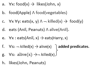
Here f and g are added predicates.

Step-2: Conversion of FOL into CNF

In First order logic resolution, it is required to convert the FOL into CNF as CNF form makes easier for resolution proofs.

Eliminate all implication (→) and rewrite

1. ∀x ¬ food(x) V likes(John, x)
2. Food(Apple) Λ food(vegetables)
3. ∀x ∀y ¬ [eats(x, y) Λ¬ killed(x)] V food(y)
4. Eats (Anil, Peanuts) Λ alive(Anil)
5. ∀x ¬ eats(Anil, x) V eats(Harry, x)
6. ∀x¬ [¬ killed(x) ] V alive(x)
7. ∀x ¬ alive(x) V ¬ killed(x)
8. Likes(John, Peanuts).

Move negation (¬)inwards and rewrite

9.     ∀x ¬ food(x) V likes(John, x)

10. food(Apple) Λ food(vegetables)

11. ∀x ∀y ¬ eats(x, y) V killed(x) V food(y)

12. eats (Anil, Peanuts) Λ alive(Anil)

13. ∀x ¬ eats(Anil, x) V eats(Harry, x)

14. ∀x ¬killed(x) ] V alive(x)

15. ∀x ¬ alive(x) V ¬ killed(x)

16. likes(John, Peanuts).

Rename variables or standardize variables

17. ∀x ¬ food(x) V likes(John, x)

18. food(Apple) Λ food(vegetables)

19. ∀y ∀z ¬ eats(y, z) V killed(y) V food(z)

20. eats (Anil, Peanuts) Λ alive(Anil)

21. ∀w¬ eats(Anil, w) V eats(Harry, w)

22. ∀g ¬killed(g) ] V alive(g)

23. ∀k ¬ alive(k) V ¬ killed(k)

24. likes(John, Peanuts).

●        Eliminate existential instantiation quantifier by elimination.
In this step, we will eliminate existential quantifier ∃, and this process is known as Skolemization. But in this example problem since there is no existential quantifier so all the statements will remain same in this step.

●        Drop Universal quantifiers.

In this step we will drop all universal quantifier since all the statements are not implicitly quantified so we don't need it.

1. ¬ food(x) V likes(John, x)
2. Food(Apple)
3. Food(vegetables)
4. ¬ eats(y, z) V killed(y) V food(z)
5. Eats (Anil, Peanuts)
6. Alive(Anil)
7. ¬ eats(Anil, w) V eats(Harry, w)
8. Killed(g) V alive(g)
9. ¬ alive(k) V ¬ killed(k)
10. Likes(John, Peanuts).

Note: Statements "food(Apple) Λ food(vegetables)" and "eats (Anil, Peanuts) Λ alive(Anil)" can be written in two separate statements.

●        Distribute conjunction ∧ over disjunction ¬.

This step will not make any change in this problem.

Step-3: Negate the statement to be proved

In this statement, we will apply negation to the conclusion statements, which will be written as ¬likes(John, Peanuts)

Step-4: Draw Resolution graph:

Now in this step, we will solve the problem by resolution tree using substitution. For the above problem, it will be given as follows:

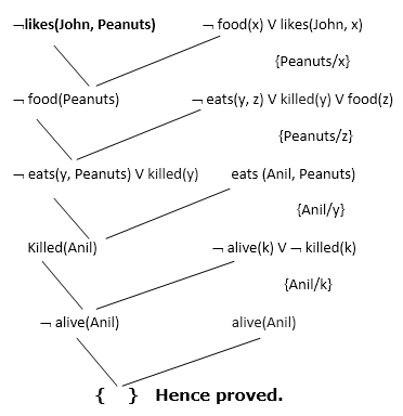
Hence the negation of the conclusion has been proved as a complete contradiction with the given set of statements.

Explanation of Resolution graph:

●        In the first step of resolution graph, ¬likes(John, Peanuts) , and likes(John, x) get resolved(cancelled) by substitution of {Peanuts/x}, and we are left with ¬ food(Peanuts)

●        In the second step of the resolution graph, ¬ food(Peanuts) , and food(z) get resolved (cancelled) by substitution of { Peanuts/z}, and we are left with ¬ eats(y, Peanuts) V killed(y) .

●        In the third step of the resolution graph, ¬ eats(y, Peanuts) and eats (Anil, Peanuts) get resolved by substitution {Anil/y}, and we are left with Killed(Anil) .

●        In the fourth step of the resolution graph, Killed(Anil) and ¬ killed(k) get resolve by substitution {Anil/k}, and we are left with ¬ alive(Anil) .

●        In the last step of the resolution graph ¬ alive(Anil) and alive(Anil) get resolved.

Key takeaway

Resolution is a theorem proving technique that proceeds by building refutation proofs, i.e., proofs by contradictions. It was invented by Mathematician John Alan Robinson in 1965.

References:

1. Elaine Rich, Kevin Knight and Shivashankar B Nair, “Artificial Intelligence”, Mc Graw Hill Publication, 2009.
2. Dan W. Patterson, “Introduction to Artificial Intelligence and Expert System”, Pearson Publication,2015.
3. Saroj Kaushik, “Artificial Intelligence”, Cengage Learning, 2011.