Unit - 5
Structured Knowledge
Basic problem-solving knowledge is structural knowledge.
It describes the connections between distinct concepts such as kind, part of, and grouping.
It is a term that describes the relationship between two or more concepts or objects.
Associative networks
A network of connections A labelled directed graph can be used to describe relational knowledge. A notion is represented by each vertex of the graph, and a relationship between concepts is represented by each label. The graph is traversed and manipulated using access and update operations. A semantic network can be thought of as a graphical representation of logical formulas. In addition, see knowledge representation.
The logical formalism Conceptual Graphs (CG) includes classes, relations, people, and quantifiers. This formalism is built on semantic networks, yet it has a direct translation to the first-order predicate logic language from which it derives its semantics. The major feature is a standardised graphical representation, which, like semantic networks, allows humans to quickly grasp the meaning of the graph. A conceptual graph is a bipartite oriented graph in which concept instances are represented by rectangles and conceptual interactions by ellipses. Oriented edges connect these vertices, indicating the existence and orientation of the relationship. When a relation has more than one edge, the edges are numbered. The figure below is an example of a graphical representation, known as Display Form (DF), of the text "a cat is on a mat."

Fig 1: Simple conceptual graph in the graphical representation DF
This sentence would be written in Linear Form (LF) using textual notation.
[Cat]-(On)-[Mat]
DF and LF are designed to be human representation (and presentation) formats. The CG Interchange Form (CGIF) is a formal language that has been defined. The sentence would be written in this language as
[Cat: *x] [Mat: *y] (On ?x ?y)
Where ?x is a reference to the declared variable and *x is a variable definition. The same sentence could be written in the same language as using syntactical shortcuts.
(On [Cat] [Mat])
The three languages' conversions are defined, as well as the direct conversion between CGIF and KIF (Knowledge Interchange Format). This example would be written in the KIF language as
Exists ((?x Cat) (?y Mat)) (On ?x ?y))
In predicate logic, all of these forms have the same semantics:
∃ x,y: Cat(x) ∧ Mat(x) ∧ on(x,y)
Predicate logic and conceptual graphs have the same expressing power. As we've seen, it's possible to construct concepts (i.e., ontology) and then use them to express specific states of affairs once more.
Key takeaway
The logical formalism Conceptual Graphs (CG) includes classes, relations, people, and quantifiers. This formalism is built on semantic networks, yet it has a direct translation to the first-order predicate logic language from which it derives its semantics.
Frames are a sort of artificial intelligence data structure that represents "stereotyped circumstances" and is used to partition knowledge into substructures. In his 1974 article "A Framework for Representing Knowledge," Marvin Minsky introduced them. Frames, which are maintained as ontologies of sets, are the basic data structure used in artificial intelligence frame language.
A frame is a record-like structure that contains a set of properties and their values to describe a physical thing. Frames are a sort of artificial intelligence data structure that splits knowledge into substructures by depicting stereotyped situations. It is made up of a set of slots and slot values. These slots can come in any shape or size. Facets are the names and values assigned to slots.
Facets are the numerous aspects of a slot machine. Facets are characteristics of frames that allow us to constrain them. When data from a certain slot is required, IF-NEEDED facts are called. A frame can have any number of slots, each of which can contain any number of facets, each of which can have any number of values. In artificial intelligence, a frame is also known as slot-filter knowledge representation.
Semantic networks gave rise to frames, which later evolved into our modern-day classes and objects. A single frame is of limited utility. A frames system is made up of a group of interconnected frames. Knowledge about an object or event can be kept in the knowledge base in the frame. The frame is a technique that is widely utilised in a variety of applications, such as natural language processing and machine vision.
Frames play an important role in knowledge representation and reasoning. They are part of structure-based knowledge representations because they were originally created from semantic networks. According to Russell and Norvig's "Artificial Intelligence: A Modern Approach", structural representations assemble "[...]facts about particular object and event types and arrange the types into a large taxonomic hierarchy analogous to a biological taxonomy".
The frame includes instructions on how to use it, what to expect next, and what to do if your expectations aren't realised. Some data in the frame remains constant, while data stored in "terminals" is more likely to change. Variables can be thought of as terminals. Top level frames provide information about the situation at hand that is always true; however, terminals do not have to be true. Their worth may fluctuate when fresh information becomes available. The same terminals may be shared by multiple frames.
Each piece of data regarding a specific frame is stored in a slot. The data may include the following:
● Facts or Data
○ Values (called facets)
● Procedures (also called procedural attachments)
○ IF-NEEDED: deferred evaluation
○ IF-ADDED: updates linked information
● Default Values
○ For Data
○ For Procedures
● Other Frames or Subframes
Key takeaway
Frames are a sort of artificial intelligence data structure that represents "stereotyped circumstances" and is used to partition knowledge into substructures.
An expert system is a computer software that can handle complex issues and make decisions in the same way as a human expert can. It does so by pulling knowledge from its knowledge base based on the user's queries, employing reasoning and inference procedures.
The expert system is a type of AI, and the first ES was created in 1970, making it the first successful artificial intelligence approach. As an expert, it solves the most difficult problems by extracting knowledge from its knowledge base. Like a human expert, the system assists in decision making for complex problems by employing both facts and heuristics.
It is so named because it comprises expert knowledge of a certain subject and is capable of solving any complex problem in that domain. These systems are tailored to a particular field, such as medicine or science.
An expert system's performance is determined on the knowledge stored in its knowledge base by the expert. The more knowledge that is stored in the KB, the better the system performs. When typing in the Google search box, one of the most common examples of an ES is a suggestion of spelling problems.
Rule based systems
A rule-based system is used in computer science to store and manipulate knowledge in order to understand data in a usable way. It's frequently utilised in artificial intelligence research and applications.
Typically, the term "rule-based system" refers to systems that have rule sets that have been handcrafted or curated by humans. This system type usually excludes rule-based systems that use automatic rule inference, such as rule-based machine learning.
Applications
The domain-specific expert system, which utilises rules to make deductions or choices, is a classic example of a rule-based system. [1] An expert system could, for example, assist a doctor in determining the correct diagnosis based on a group of symptoms or selecting tactical actions in a game.
Lexical analysis, compiling or interpreting computer programmes, and natural language processing can all benefit from rule-based systems.
From a beginning collection of data and rules, rule-based programming seeks to derive execution instructions. This is a less direct approach than imperative programming languages, which list execution stages in a sequential order.
Constructions
The following are the four basic components of a rule-based system:
● A rule base is a sort of knowledge base that has a list of rules.
● Based on the interplay of input and the rule base, an inference engine or semantic reasoner infers knowledge or takes action. The following match-resolve-act cycle is used by the interpreter to run a production system programme:
● Match - The left-hand sides of all productions are matched against the contents of working memory in this first phase. As a result, a conflict set containing instantiations of all satisfied productions is obtained. A production instantiation is an ordered list of working memory items that fulfils the production's left-hand side.
● Conflict - resolution - In the second phase, one of the conflict set's production instantiations is chosen for execution. The interpreter comes to a halt if no productions are satisfied.
● Act - The actions of the production chosen in the conflict-resolution phase are carried out in this third phase. These actions have the potential to alter the contents of working memory. Execution returns to the first phase at the end of this phase.
● Working memory that is only active for a short period of time.
● Input and output signals are received and sent through a user interface or other connection to the outside world.
Key takeaway
An expert system is a computer software that can handle complex issues and make decisions in the same way as a human expert can.
A rule-based system is used in computer science to store and manipulate knowledge in order to understand data in a usable way. It's frequently utilised in artificial intelligence research and applications.
Decision Tree is a supervised learning technique that may be used to solve both classification and regression problems, however it is most commonly employed to solve classification issues. Internal nodes represent dataset attributes, branches represent decision rules, and each leaf node provides the conclusion in this tree-structured classifier.
The Decision Node and the Leaf Node are the two nodes of a Decision tree. Leaf nodes are the output of those decisions and do not contain any more branches, whereas Decision nodes are used to make any decision and have several branches.
The decisions or tests are made based on the characteristics of the given dataset.
It's a graphical depiction for obtaining all feasible solutions to a problem/decision depending on certain parameters.
It's termed a decision tree because, like a tree, it starts with the root node and grows into a tree-like structure with additional branches. We utilise the CART algorithm, which stands for Classification and Regression Tree algorithm, to form a tree.
A decision tree simply asks a question and divides the tree into subtrees based on the answer (Yes/No).
A decision tree's general structure is seen in the diagram below:
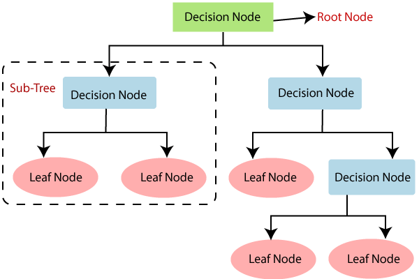
Fig 2: Decision tree
Decision tree terminology
Root node - The decision tree begins at the root node. It represents the full dataset, which is then split into two or more homogeneous groups.
Leaf node - Leaf nodes are the last output nodes, and the tree cannot be further segmented once a leaf node has been obtained.
Splitting - Splitting is the process of separating a decision node/root node into sub-nodes based on the conditions specified.
Branch / Sub tree - A tree that has been split in half.
Pruning - Pruning is the procedure of pruning a tree to remove undesired branches.
Parent / child node - The parent node is the tree's root node, while the child nodes are the tree's other nodes.
Working of Decision tree algorithm
The procedure for determining the class of a given dataset in a decision tree starts at the root node of the tree. This algorithm checks the values of the root attribute with the values of the record (actual dataset) attribute and then follows the branch and jumps to the next node based on the comparison.
The algorithm compares the attribute value with the other sub-nodes and moves on to the next node. It repeats the process until it reaches the tree's leaf node. The following algorithm can help you understand the entire process:
Step-1: Begin the tree with the root node, says S, which contains the complete dataset.
Step-2: Find the best attribute in the dataset using Attribute Selection Measure (ASM).
Step-3: Divide the S into subsets that contains possible values for the best attributes.
Step-4: Generate the decision tree node, which contains the best attribute.
Step-5: Recursively make new decision trees using the subsets of the dataset created in step -3. Continue this process until a stage is reached where you cannot further classify the nodes and called the final node as a leaf node.
Why do we use decision trees?
Machine learning uses a variety of methods, therefore picking the optimal approach for the given dataset and problem is the most important thing to remember while building a machine learning model. The following are two reasons to use the Decision Tree:
Decision Trees are designed to mirror human thinking abilities when making decisions, making them simple to comprehend.
Because the decision tree has a tree-like form, the rationale behind it is simple to comprehend.
Key takeaway
Decision Tree is a supervised learning technique that may be used to solve both classification and regression problems, however it is most commonly employed to solve classification issues.
The blackboard architecture is a strong expert system architecture and distributed problem-solving approach. It can answer problems with a significant amount of different, erroneous, and incomplete knowledge. A common data region called the blackboard, a number of independent knowledge sources, and a control unit called the scheduler make up the basic blackboard architecture. It allows for the organisation of the application of this information as well as the necessary interaction between the sources of this knowledge.
A blackboard system's key advantages are its control flexibility and ability to incorporate many types of knowledge representation and inferencing techniques. A blackboard system can include, for example, a production rule system or a frame-based system.
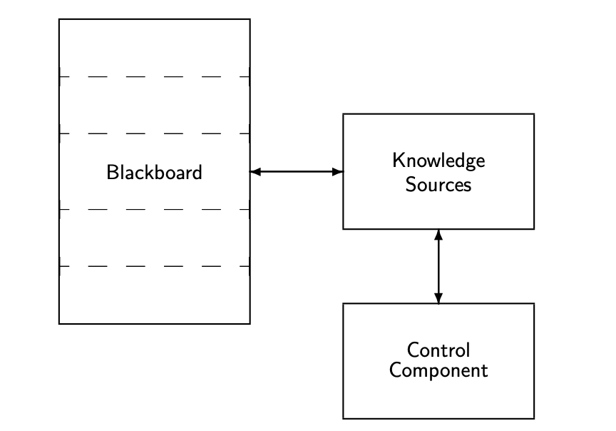
Fig 3: Basic Components of the Blackboard Model
The blackboard system is made up of three parts:
● Blackboard (BB),
● Knowledge sources (KSs), and
● Control unit.
Blackboard
It is the element of the system that stores knowledge that is accessible to all KSs. It's a global data structure for organising problem-solving data and coordinating communications between KSs. Input data, partial outcomes, hypotheses, options, and the final solution might all be posted on the BB. The BB is used to facilitate interaction amongst the KSs. A blackboard can be divided into an infinite number of sub-blackboards, which are also known as planes or panels. That is, a BB can be subdivided into multiple BB levels, each of which corresponds to a distinct part of the solution process. As a result, the objects can be arranged into multiple levels of study in a hierarchical manner.
This split, however, is optional and is determined by the nature of the application. A list of attribute values can be used to store an object. On the BB, an event is produced or changed that specifies the occurrence of a specific condition. It's used to figure out which KSs are allowed to participate in the problem-solving process at any particular time. A single BB event can set off a cascade of KSs.
A certainty factor can be assigned to each BB entry. This is one method the system deals with knowledge ambiguity. The blackboard technique assures that each KS and the partial solutions identified so far have a consistent interface. As a result, KSs are rather self-contained.
Knowledge source
Knowledge sources are domain knowledge modules that self-select. Each knowledge source can be thought of as a stand-alone application that specialises in processing a specific type of data or knowledge in a specific domain. Each information source should be able to determine whether or not it should participate in the problem-solving process at any given time. In a blackboard system, the knowledge sources are segregated and independent. Each has its own working procedures or regulations, as well as a private data structure. It contains information required for the knowledge source to run correctly. The action element of a knowledge source is responsible for actual issue solving and BB modifications.
Control unit
The problem-solving process is guided by an explicit control mechanism that allows KSs to respond opportunistically to changes in the blackboard database. The control mechanism decides what to do based on the state of the blackboard and the set of activated KSs.
A blackboard system employs incremental reasoning, which means that the answer is constructed one step at a time. The system can do the following at each step:
● Execute any triggered KS
● Choose a different focus of attention, on the basis of the state of the solution.
The currently running KS activation generates events as it contributes to the blackboard in a normal control way. These events are kept (and maybe ranked) until the KS activation in progress is finished. The control components then use the events to activate and trigger the KSs. The KS activations are prioritised, and the one that is most appropriate for execution is chosen. This cycle will continue until the issue has been resolved.
Because Blackboard systems provide a number of control mechanisms and algorithms, application developers have a selection of opportunistic control techniques to choose from.
Key takeaway
The blackboard architecture is a strong expert system architecture and distributed problem-solving approach. It can answer problems with a significant amount of different, erroneous, and incomplete knowledge.
Yet another research area in AI, neural networks, is inspired from the natural neural network of human nervous system.
What are Artificial Neural Networks (ANNs)?
The inventor of the first neurocomputer, Dr. Robert Hecht-Nielsen, defines a neural network as −
"...a computing system made up of a number of simple, highly interconnected processing elements, which process information by their dynamic state response to external inputs.”
Basic Structure of ANNs
The idea of ANNs is based on the belief that working of human brain by making the right connections, can be imitated using silicon and wires as living neurons and dendrites.
The human brain is composed of 86 billion nerve cells called neurons. They are connected to other thousand cells by Axons. Stimuli from external environment or inputs from sensory organs are accepted by dendrites. These inputs create electric impulses, which quickly travel through the neural network. A neuron can then send the message to other neuron to handle the issue or does not send it forward.
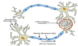
Fig 4: Neurons
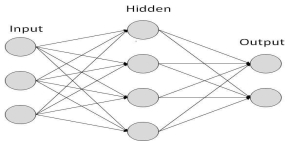
ANNs are composed of multiple nodes, which imitate biological neurons of human brain. The neurons are connected by links and they interact with each other. The nodes can take input data and perform simple operations on the data. The result of these operations is passed to other neurons. The output at each node is called its activation or node value.
Each link is associated with weight. ANNs are capable of learning, which takes place by altering weight values. The following illustration shows a simple ANN −
Types of Artificial Neural Networks
There are two Artificial Neural Network topologies – Feed Forward and Feedback.
Feed Forward ANN
In this ANN, the information flow is unidirectional. A unit sends information to other unit from which it does not receive any information. There are no feedback loops. They are used in pattern generation/recognition/classification. They have fixed inputs and outputs.
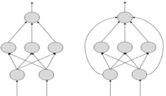
Fig 5: Feedforward ANN
Feed Back ANN
Here, feedback loops are allowed. They are used in content addressable memories.
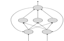
Fig 6: Feedback ANN
Working of ANNs
In the topology diagrams shown, each arrow represents a connection between two neurons and indicates the pathway for the flow of information. Each connection has a weight, an integer number that controls the signal between the two neurons.
If the network generates a “good or desired” output, there is no need to adjust the weights. However, if the network generates a “poor or undesired” output or an error, then the system alters the weights in order to improve subsequent results.
Machine Learning in ANNs
ANNs are capable of learning and they need to be trained. There are several learning strategies −
● Supervised Learning − It involves a teacher that is scholar than the ANN itself. For example, the teacher feeds some example data about which the teacher already knows the answers.
For example, pattern recognizing. The ANN comes up with guesses while recognizing. Then the teacher provides the ANN with the answers. The network then compares it guesses with the teacher’s “correct” answers and makes adjustments according to errors.
● Unsupervised Learning − It is required when there is no example data set with known answers. For example, searching for a hidden pattern. In this case, clustering i.e. dividing a set of elements into groups according to some unknown pattern is carried out based on the existing data sets present.
● Reinforcement Learning − This strategy built on observation. The ANN makes a decision by observing its environment. If the observation is negative, the network adjusts its weights to be able to make a different required decision the next time.
Back Propagation Algorithm
It is the training or learning algorithm. It learns by example. If you submit to the algorithm the example of what you want the network to do, it changes the network’s weights so that it can produce desired output for a particular input on finishing the training.
Back Propagation networks are ideal for simple Pattern Recognition and Mapping Tasks.
Bayesian Networks (BN)
These are the graphical structures used to represent the probabilistic relationship among a set of random variables. Bayesian networks are also called Belief Networks or Bayes Nets. BNs reason about uncertain domain.
In these networks, each node represents a random variable with specific propositions. For example, in a medical diagnosis domain, the node Cancer represents the proposition that a patient has cancer.
The edges connecting the nodes represent probabilistic dependencies among those random variables. If out of two nodes, one is affecting the other then they must be directly connected in the directions of the effect. The strength of the relationship between variables is quantified by the probability associated with each node.
There is an only constraint on the arcs in a BN that you cannot return to a node simply by following directed arcs. Hence the BNs are called Directed Acyclic Graphs (DAGs).
BNs are capable of handling multivalued variables simultaneously. The BN variables are composed of two dimensions −
● Range of prepositions
● Probability assigned to each of the prepositions.
Consider a finite set X = {X1, X2, …,Xn} of discrete random variables, where each variable Xi may take values from a finite set, denoted by Val(Xi). If there is a directed link from variable Xi to variable, Xj, then variable Xi will be a parent of variable Xj showing direct dependencies between the variables.
The structure of BN is ideal for combining prior knowledge and observed data. BN can be used to learn the causal relationships and understand various problem domains and to predict future events, even in case of missing data.
Building a Bayesian Network
A knowledge engineer can build a Bayesian network. There are a number of steps the knowledge engineer needs to take while building it.
Example problem − Lung cancer. A patient has been suffering from breathlessness. He visits the doctor, suspecting he has lung cancer. The doctor knows that barring lung cancer, there are various other possible diseases the patient might have such as tuberculosis and bronchitis.
Gather Relevant Information of Problem
● Is the patient a smoker? If yes, then high chances of cancer and bronchitis.
● Is the patient exposed to air pollution? If yes, what sort of air pollution?
● Take an X-Ray positive X-ray would indicate either TB or lung cancer.
Identify Interesting Variables
The knowledge engineer tries to answer the questions −
● Which nodes to represent?
● What values can they take? In which state can they be?
For now let us consider nodes, with only discrete values. The variable must take on exactly one of these values at a time.
Common types of discrete nodes are −
● Boolean nodes − They represent propositions, taking binary values TRUE (T) and FALSE (F).
● Ordered values − A node Pollution might represent and take values from {low, medium, high} describing degree of a patient’s exposure to pollution.
● Integral values − A node called Age might represent patient’s age with possible values from 1 to 120. Even at this early stage, modeling choices are being made.
Possible nodes and values for the lung cancer example −
Node Name | Type | Value | Nodes Creation |
Polution | Binary | {LOW, HIGH, MEDIUM} | 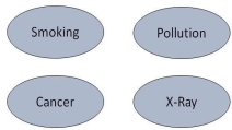 |
Smoker | Boolean | {TRUE, FASLE} | |
Lung-Cancer | Boolean | {TRUE, FASLE} | |
X-Ray | Binary | {Positive, Negative} |
Create Arcs between Nodes
Topology of the network should capture qualitative relationships between variables.
For example, what causes a patient to have lung cancer? - Pollution and smoking. Then add arcs from node Pollution and node Smoker to node Lung-Cancer.
Similarly if patient has lung cancer, then X-ray result will be positive. Then add arcs from node Lung-Cancer to node X-Ray.
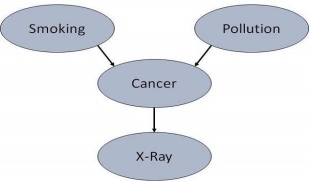
Specify Topology
Conventionally, BNs are laid out so that the arcs point from top to bottom. The set of parent nodes of a node X is given by Parents(X).
The Lung-Cancer node has two parents (reasons or causes): Pollution and Smoker, while node Smoker is an ancestor of node X-Ray. Similarly, X-Ray is a child (consequence or effects) of node Lung-Cancer and successor of nodes Smoker and Pollution.
Conditional Probabilities
Now quantify the relationships between connected nodes: this is done by specifying a conditional probability distribution for each node. As only discrete variables are considered here, this takes the form of a Conditional Probability Table (CPT).
First, for each node we need to look at all the possible combinations of values of those parent nodes. Each such combination is called an instantiation of the parent set. For each distinct instantiation of parent node values, we need to specify the probability that the child will take.
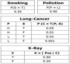
For example, the Lung-Cancer node’s parents are Pollution and Smoking. They take the possible values = { (H,T), ( H,F), (L,T), (L,F)}. The CPT specifies the probability of cancer for each of these cases as <0.05, 0.02, 0.03, 0.001> respectively.
Each node will have conditional probability associated as follows −
Applications of Neural Networks
They can perform tasks that are easy for a human but difficult for a machine −
● Aerospace − Autopilot aircrafts, aircraft fault detection.
● Automotive − Automobile guidance systems.
● Military − Weapon orientation and steering, target tracking, object discrimination, facial recognition, signal/image identification.
● Electronics − Code sequence prediction, IC chip layout, chip failure analysis, machine vision, voice synthesis.
● Financial − Real estate appraisal, loan advisor, mortgage screening, corporate bond rating, portfolio trading program, corporate financial analysis, currency value prediction, document readers, credit application evaluators.
● Industrial − Manufacturing process control, product design and analysis, quality inspection systems, welding quality analysis, paper quality prediction, chemical product design analysis, dynamic modeling of chemical process systems, machine maintenance analysis, project bidding, planning, and management.
● Medical − Cancer cell analysis, EEG and ECG analysis, prosthetic design, transplant time optimizer.
● Speech − Speech recognition, speech classification, text to speech conversion.
● Telecommunications − Image and data compression, automated information services, real-time spoken language translation.
● Transportation − Truck Brake system diagnosis, vehicle scheduling, routing systems.
● Software − Pattern Recognition in facial recognition, optical character recognition, etc.
● Time Series Prediction − ANNs are used to make predictions on stocks and natural calamities.
● Signal Processing − Neural networks can be trained to process an audio signal and filter it appropriately in the hearing aids.
● Control − ANNs are often used to make steering decisions of physical vehicles.
● Anomaly Detection − As ANNs are expert at recognizing patterns, they can also be trained to generate an output when something unusual occurs that misfits the pattern.
Key takeaway
The idea of ANNs is based on the belief that working of human brain by making the right connections, can be imitated using silicon and wires as living neurons and dendrites.
There are several ways to frame this definition, but largely there are three main known categories: supervised learning, unsupervised learning, and reinforcement learning.
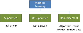
Fig 7: Types of Learning
In a world filled by artificial intelligence, machine learning, and over-zealous talk about both, it is interesting to learn to understand and define the types of machine learning we may encounter. For the average computer user, this may take the form of knowing the forms of machine learning and how they can exhibit themselves in applications we use.
And for the practitioners designing these applications, it’s important to know the styles of machine learning so that for any given task you can face, you can craft the proper learning environment and understand why what you did succeeded.
- Supervised Learning
Supervised learning is the most common model for machine learning. It is the easiest to grasp and the quickest to execute. It is quite close to training a child through the use of flash cards.
Supervised learning is also defined as task-oriented because of this. It is highly focused on a single task, feeding more and more examples to the algorithm before it can reliably perform on that task.
There are two major types of supervised learning problems: classification that involves predicting a class mark and regression that involves predicting a numerical value.
● Classification: Supervised learning problem that involves predicting a class mark.
● Regression: Supervised learning problem that requires predicting a numerical mark.
Both classification and regression problems can have one or more input variables and input variables may be any data form, such as numerical or categorical.
2. Unsupervised Learning
Unsupervised learning is very much the opposite of supervised learning. It features no marks. Instead, our algorithm will be fed a lot of data and provided the tools to understand the properties of the data. From there, it can learn to group, cluster, and/or arrange the data in a way so that a person (or other intelligent algorithm) can come in and make sense of the newly arranged data.
There are several forms of unsupervised learning, but there are two key problems that are mostly faced by a practitioner: they are clustering that involves identifying groups in the data and density estimation that involves summarising the distribution of data.
● Clustering: Unsupervised learning problem that involves finding groups in data.
● Density Estimation: Unsupervised learning problem that involves summarizing the distribution of data.
3. Reinforcement Learning
Reinforcement learning is fairly different when compared to supervised and unsupervised learning. Where we can clearly see the relationship between supervised and unsupervised (the existence or absence of labels), the relationship to reinforcement learning is a little murkier. Some people attempt to tie reinforcement learning closer to the two by defining it as a form of learning that relies on a time-dependent sequence of labels, however, my opinion is that that actually makes things more complicated.
For any reinforcement learning challenge, we need an agent and an environment as well as a way to link the two via a feedback loop. To link the agent to the world, we give it a collection of actions that it can take that affect the environment. To link the environment to the agent, we make it continually issue two signals to the agent: an updated state and a reward (our reinforcement signal for behavior) (our reinforcement signal for behavior).
Key takeaway:
● Supervised learning is the most common model for machine learning. It is the easiest to grasp and the quickest to execute.
● Unsupervised learning is very much the opposite of supervised learning. It features no marks. Instead, our algorithm will be fed a lot of data and provided the tools to understand the properties of the data.
● Reinforcement learning is fairly different when compared to supervised and unsupervised learning.
Learning can be performed in a variety of ways, including memory of knowledge, being informed, or studying examples such as problem solving. Learning necessitates the creation of new knowledge structures from some form of input stimulation. This new information must then be incorporated into a knowledge base and put to some kind of test to see if it is useful. Testing implies that the knowledge be applied to a task from which meaningful feedback may be gained, with the feedback providing some indication of the accuracy and utility of the newly learned knowledge.
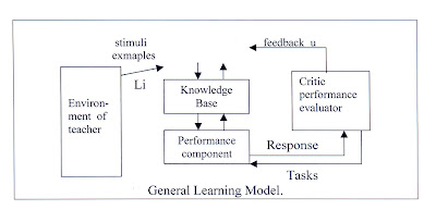
Fig 8: General Learning Model
The environment has been integrated as an element of the overall learner system in the general learning model represented in fig. The environment can be viewed as either a random form of nature or a more planned training source like a teacher who delivers carefully selected training examples for the learner component. The type of environment used will be determined by the learning paradigm. In any scenario, some form of representation language between the learner and the environment must be assumed. It's possible that the language uses the same representation strategy as the knowledge base (such as a form of predicate calculus). The single representation trick is applied when they are chosen to be the same. Because no transformation between two or more different representations is required, this usually leads to a simpler implementation.
The environment for certain systems could be a user typing on a keyboard. To replicate a specific environment, other systems will employ programme modules. In progressively more realistic scenarios, the system will include real physical sensors that interact with the outside world.
Physical stimuli or descriptive, symbolic training examples may be used as inputs to the learner component. The knowledge structures in the knowledge base are created and modified using the information supplied to the learner component. The performance component uses this same knowledge to carry out some tasks, such as solving a problem while playing a game or identifying instances of a concept.
When given a task, the performance component responds with a response that describes how it performed the task. After that, the critic module compares this response to an ideal one.
The critic module then sends feedback to the learner component, indicating whether or not the performance was acceptable, so that the structures in the knowledge base can be modified. With the updates to the knowledge base, the system's performance will have increased if proper learning was completed.
The cycle described above can be repeated several times until the system's performance has reached an acceptable level, a known learning goal has been met, or changes in the knowledge base have stopped occurring after a certain number of training examples have been observed.
In addition to the type of representation utilised, there are several other crucial elements that influence a system's ability to learn. The types of training supplied, the form and quantity of any prior background knowledge, the type of feedback provided, and the learning algorithms utilised are all factors to consider.
The sort of training utilised in a system, much as in humans, can have a significant impact on performance. Training can include a random selection of instances or examples that have been deliberately chosen and ordered for presentation. The examples could be positive examples of a topic or task being learnt, bad examples, or a mix of both positive and negative examples. The instances may be tightly focused, containing just pertinent data, or they may contain a wide range of facts and details, including irrelevant information.
Many types of learning can be described as a search for hypotheses or solutions in a space of possibilities. To improve the efficiency of learning. This search method must be limited or the search space must be reduced. One way to do this is to leverage prior information to narrow the search space or to perform control operations that limit the search process.
Key takeaway
Learning can be performed in a variety of ways, including memory of knowledge, being informed, or studying examples such as problem solving. Learning necessitates the creation of new knowledge structures from some form of input stimulation.
Learning through Induction We have a collection of xi, f (xi) for 1in in supervised learning, and our goal is to determine 'f' using an adaptive approach. It's a machine learning method for inferring rules from facts or data. In logic, conditional or antecedent reasoning is the process of reasoning from the specific to the general. Theoretical studies in machine learning mostly concern supervised learning, a sort of inductive learning. An algorithm is provided with samples that are labeled in a useful way in supervised learning.
Inductive learning techniques, such as artificial neural networks, allow the real robot to learn simply from data that has already been collected. Another way is to let the bot learn everything in his environment by inducing facts from it. Inductive learning is the term for this type of learning. Finally, you may train the bot to evolve across numerous generations and improve its performance.
f(x) is the target function
An example is a pair [x, f(x)]
Some practical examples of induction are:
● Credit risk assessment.
○ The x is the property of the customer.
○ The f(x) is credit approved or not.
● Disease diagnosis.
○ The x are the properties of the patient.
○ The f(x) is the disease they suffer from.
● Face recognition.
○ The x are bitmaps of people’s faces.
○ The f(x) is to assign a name to the face.
● Automatic steering.
○ The x are bitmap images from a camera in front of the car.
○ The f(x) is the degree the steering wheel should be turned.
Two perspectives on inductive learning:
● Learning is the removal of uncertainty. Data removes some of the uncertainty. We are removing more uncertainty by selecting a class of hypotheses.
● Learning is guessing a good and small hypothesis class. It necessitates speculation. Because we don't know the answer, we'll have to rely on trial and error. You don't need to learn if you're confident in your domain knowledge. But we're not making educated guesses.
Generalization’s major purpose is to improve the AI system's performance on test data. Transfer Learning, on the other hand, entails training the system on some tasks in order to increase its performance on others. While these two approaches may appear to be very different in reality, they both have the same goal: forcing a neural network or other machine learning algorithm to acquire relevant concepts in one context in order to perform better in another.
Generalization is a term used in machine learning to describe how well a trained model can categorise or forecast unknown data. When you train a generalised machine learning model, you ensure that it works for any subset of unknown data. When we train a model to distinguish between dogs and cats, for example. If the model is given a dataset of dogs photos containing only two breeds, it may perform well. However, when it is examined by other dog breeds, it may receive a poor classification score. This problem can cause an unknown dataset to categorise an actual dog image as a cat. As a result, data diversity is a critical aspect in making a solid forecast.
In the example above, the model may achieve an 85 percent performance score when only two dog breeds are tested, and a 70 percent performance score when all breeds are trained. However, if it is evaluated by an unknown dataset with all breed dogs, the first may have a relatively low score (e.g. 45 percent). This for the latter can remain intact because it has been trained using a large amount of data diversity that includes all potential breeds.
It's important to remember that data diversity isn't the only factor to consider while developing a generalised model. It can be caused by the nature of a machine learning algorithm or by a poorly configured hyper-parameter. All determinant factors are explained in this essay. To ensure generalisation, several procedures (regularisation) can be used during model training. But first, we'll go into bias, variation, and underfitting and overfitting.
They're also linked to the difficulties of underfitting and overfitting:

Underfitting occurs when the model's capacity is insufficient or the model has not been trained long enough to memorise crucial characteristics. Overfitting occurs when the model is too large and/or trained for too long, causing it to over adjust to the training data. This research demonstrates that deep neural networks can quickly memorise the whole training dataset. With this in mind, a great deal of research is being done on regularisation approaches with the goal of resolving these problems.
Specialization
In 2018, York University added an Artificial Intelligence (AI) Specialization to its Master of Science in Computer Science degree. While AI-based research continues to be pursued in the main stream of the programme, students in this specialisation take six graduate courses in their first two terms, at least five of which are in the area of AI. In addition, under the supervision of faculty members and in partnership with corporate or public sector partners, students perform a research project that applies AI to a practical problem. With this understanding, our graduates will be able to successfully use AI approaches in a variety of industries.
The Vector Institute has acknowledged our AI Specialization, allowing our students to apply for Vector Scholarships in Artificial Intelligence.
Note that the AI specialisation is intended to provide specific training for applying AI concepts in the workplace, but it is not eligible for future PhD study because it is non-thesis. The MSc in Computer Science programme is for those who want to do AI-based research in a thesis programme.
The student will be responsible for finding an internship for their research project. Through networking events and the Vector Digital Talent Hub, the Vector Institute aids the process by allowing students in this programme to contact potential employers.
Key takeaway
Generalization’s major purpose is to improve the AI system's performance on test data. Transfer Learning, on the other hand, entails training the system on some tasks in order to increase its performance on others.
If we have an example set with the attributes Place type, weather, location, decision, and seven examples, our objective is to construct a set of rules to determine what the decision is under what conditions.
Some practical examples of induction are:
Credit risk assessment.
● The x is the property of the customer.
● The f(x) is credit approved or not.
Disease diagnosis.
● The x is the characteristics of a given patient.
● The f(x) is the patient’s disease.
Face recognition.
● The x are bitmaps of the faces we want to recognize.
● The f(x) is a name assigned to that face.
Automatic steering (autonomous driving).
● The x is bitmap images from a camera in front of the car.
● The f(x) is the degree to which the steering wheel should be turned.
Application
Inductive Learning is not appropriate in some instances. It's crucial to know when to utilise supervised machine learning and when not to.
The following four scenarios may benefit from inductive learning:
● Problems for which there is no human competence. When people don't know the answer to a problem, they can't develop a programme to solve it. These are places that are ideal for investigation.
● Humans are capable of completing the task, but no one knows how. Humans can do things that computers can't or can't do well in some instances. Bike riding and car driving are two examples.
● Problems with the desired function changing frequently. Humans could define the problem and design a programme to solve it, but the problem is constantly changing. It is not cost-effective. One example is the stock market.
● Problems requiring a unique function for each user. It is not cost-effective to write custom software for each user. Consider Netflix or Amazon for movie or book recommendations.
References:
- Elaine Rich, Kevin Knight and Shivashankar B Nair, “Artificial Intelligence”, Mc Graw Hill Publication, 2009.
- Dan W. Patterson, “Introduction to Artificial Intelligence and Expert System”, Pearson Publication,2015.
- Saroj Kaushik, “Artificial Intelligence”, Cengage Learning, 2011.