Unit - 4
Artificial Neural Networks
Biological neural networks establish the structure of the human brain, and the phrase "Artificial Neural Network" is taken from them. Artificial neural networks, like the human brain, have neurons that are coupled to one another in various layers of the networks. Nodes are the name for these neurons.
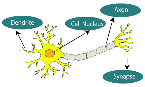
Fig 1: Neurons
The diagram seen here is a typical Biological Neural Network diagram.
The standard Artificial Neural Network resembles the illustration below.
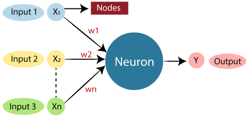
Fig 2: ANN
In Artificial Neural Networks, dendrites from biological neural networks represent inputs, cell nuclei represent nodes, synapse represent weights, and axon represent output.
In the science of artificial intelligence, an Artificial Neural Network seeks to duplicate the network of neurons that make up a human brain so that computers can understand things and make judgments in a human-like fashion. Computers are programmed to act like interconnected brain cells in order to create an artificial neural network.
The human brain contains approximately 1000 billion neurons. Each neuron has a number of association points ranging from 1,000 to 100,000. Data is stored in the human brain in such a way that it may be spread, and we can pull multiple pieces of this data from our memory at the same time if needed. The human brain, we may say, is made up of incredible parallel processors.
Consider the example of a digital logic gate that receives an input and produces an output to better understand the artificial neural network. The "OR" gate accepts two inputs. If one or both inputs are "On," the output will be "On." If both inputs are "Off," the output will be "Off." In this case, the output is determined by the input. Our brains don't work in the same way. Because our brain's neurons are "learning," the output to input connections is constantly changing.
Architectures
To comprehend the concept of artificial neural network architecture, we must first comprehend what a neural network is made up of. To describe a neural network that is made up of a large number of artificial neurons called units that are stacked in layers. Let's take a look at the various layers that may be found in an artificial neural network.
The Artificial Neural Network is made up of three layers:
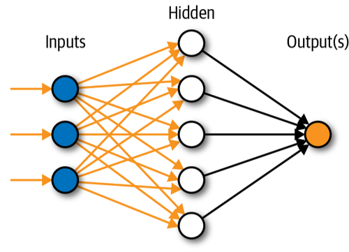
Fig 3: Architecture of ANN
- Input layer
It accepts inputs in a variety of formats specified by the programmer, as the name implies.
2. Hidden layer
Between the input and output layers is a concealed layer. It does all the math to uncover hidden features and patterns.
3. Output layer
The input goes through a series of transformations using the hidden layer, which finally results in output that is conveyed using this layer.
The artificial neural network takes input and computes the weighted sum of the inputs and includes a bias. This computation is represented in the form of a transfer function.
Advantages
● Parallel processing capability:
Artificial neural networks have a numerical value that allows them to accomplish multiple tasks at once.
● Storing data on the entire network:
Traditional programming data is saved across the entire network, not in a database. The network continues to function despite the loss of a few pieces of data in one location.
● Capability to work with incomplete knowledge:
Even with insufficient data, after ANN training, the information may produce output. The relevance of missing data is what causes the performance loss in this case.
● Having a memory distribution:
It is critical to determine the examples and to stimulate the network according to the intended output by displaying these examples to the network if the ANN is to be able to adapt.
● Having fault tolerance:
The loss of one or more ANN cells does not prevent the network from producing output, and this feature makes the network fault-tolerant.
Disadvantages
● Assurance of proper network structure:
The structure of artificial neural networks can be determined in a variety of ways. Experience, trial, and error are used to create the ideal network structure.
● Unrecognized behavior of the network:
It is ANN's most important problem. When ANN creates a testing solution, it does not explain why or how it was created. It erodes the network's trustworthiness.
● Hardware dependence:
Artificial neural networks, due to their structure, require computers with parallel processing power. As a result, the equipment's manifestation is contingent.
● Difficulty of showing the issue to the network:
ANNs are capable of working with numerical data. Before introducing problems to ANN, they must be transformed into numerical values. The presentation mechanism that must be resolved here will have a direct impact on the network's performance. It is dependent on the user's capabilities.
● The duration of the network is unknown:
The network is reduced to a specified error value, which does not provide us the best outcomes.
Key takeaway
Neural networks are mathematical models that use learning algorithms inspired by the brain to store information.
A major focus of machine-learning research is to automatically learn to recognize complex patterns and make intelligent decisions based on data.
Neural networks are a popular framework to perform machine learning, but there are many other machine-learning methods, such as logistic regression, and support vector machines.
Frank Rosenblatt introduced Perceptron in 1957. Based on the original MCP neuron, he created a Perceptron learning rule. A Perceptron is a supervised learning technique for binary classifiers. This approach allows neurons to learn and process individual components in the training set.
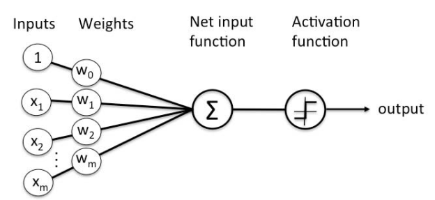
Fig 4: Perceptron
A linear decision boundary is used by the perceptron to partition the input data. Another supervised learning approach known as support vector classifiers performs a similar procedure, which you can learn more about in our full post here.
The perceptron assigns weights to a set of scalar input features as well as a constant 'bias' term. The weights and inputs are combined in a linear fashion. After that, the linear combination is fed via an activation function, which decides which state (or class) the inputs belong to.
Categories
Perceptrons are divided into two categories: single layer and multilayer.
Single layer - Single layer perceptrons can only learn patterns that are linearly separable.
Multilayer - The processing power of multilayer perceptrons or feedforward neural networks with two or more layers is increased.
In order to build a linear decision boundary, the Perceptron algorithm learns the weights for the input signals.
You can now tell the difference between the two linearly separable classes +1 and -1.
Activation function for perceptron
The perceptron model's chosen activation function is a step function that, depending on the value of the linear combination, outputs one of two distinct values (three in the case of the Sign function below).
The Heaviside function and the Sign function are two popular step functions in perceptrons.
The following is the Heaviside function (named after Oliver Heaviside):

It states to return 0 if the specified linear combination is less than 0 and 1 if it is greater than 0.
The following is the Sign function:

It says to return -1 if the specified linear combination is less than 0, 0 if it is 0, and +1 if it is greater than 0.
Key takeaway
A Perceptron is a supervised learning technique for binary classifiers. This approach allows neurons to learn and process individual components in the training set.
Gradient descent is a well-known optimization approach for training machine learning models and neural networks. These models learn over time with the use of training data, and the cost function within gradient descent functions as a barometer, assessing its correctness with each iteration of parameter updates. The model will continue to change its parameters until the function is close to or equal to zero, resulting in the least feasible error. Machine learning models can be useful tools for artificial intelligence (AI) and computer science applications once they are adjusted for accuracy.
Gradient Descent is a backpropagation phase method in which the goal is to continually resample the gradient of the model's parameter in the opposite direction depending on the weight w, updating consistently until the global minimum of function J is reached (w).
To put it another way, we minimise the cost function, J, by using gradient descent (w).
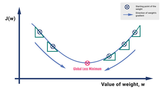
Fig 5: How Gradient Descent works for one parameter, w
A steep mountain with a base that touches the water may be used as an analogy. We presume that a person's objective is to descend to sea level. To attain the goal, the person should ideally take one step at a time. A negative gradient runs through each step (Note: the value can be of different magnitude). The hiker goes down until he reaches the bottom or reaches a point where there is no more room to go down.
Types of Gradient Descent
Gradient descent is divided into three categories, which differ mostly in the quantity of data they use:
BATCH GRADIENT DESCENT
Batch gradient descent, also known as vanilla gradient descent, evaluates the error for each example in the training dataset, but the model is updated only after all of the training instances have been reviewed. This entire procedure is referred to as a training period since it resembles a cycle.
Batch gradient descent has a number of advantages, including being computationally cheap and producing a stable error gradient and convergence. The stable error gradient might occasionally result in a state of convergence that isn't the best the model can accomplish, which is one of the downsides. It also necessitates the algorithm having access to the complete training dataset in memory.
STOCHASTIC GRADIENT DESCENT
Stochastic gradient descent (SGD), on the other hand, accomplishes this for each training sample inside the dataset, updating the parameters one by one. This can make SGD faster than batch gradient descent, depending on the situation. One advantage is the frequent updates allow us to have a pretty detailed rate of improvement.
The frequent updates, on the other hand, take longer to compute than the batch gradient descent method. Furthermore, the frequency of those updates might generate noisy gradients, causing the error rate to leap about rather than gradually reducing.
MINI-BATCH GRADIENT DESCENT
Because it combines the ideas of SGD and batch gradient descent, mini-batch gradient descent is the preferred method. It simply divides the training dataset into small batches and updates each batch separately. This strikes a balance between stochastic gradient descent's robustness and batch gradient descent's efficiency.
Mini-batch sizes typically range from 50 to 256, but like with any other machine learning technique, there is no hard and fast rule because it varies depending on the application. This is the most frequent type of gradient descent in deep learning and is the go-to technique when training a neural network.
The Delta Rule
In an artificial neural network, the delta rule is a type of backpropagation that aids in the refinement of the machine learning/artificial intelligence network by forming associations between input and output with different layers of artificial neurons. The Delta learning rule is another name for the Delta rule.
Backpropagation is the process of using a gradient approach to recalculate input weights for artificial neurons. The difference between a target activation and an obtained activation is used in delta learning to accomplish this. Network connections are balanced using a linear activation function. Another way to explain the Delta rule is that it does gradient descent learning using an error function.
The Delta rule is a type of backpropagation used in machine learning and neural network contexts to refine connectionist ML/AI networks by connecting inputs and outputs with layers of artificial neurons.
The Delta learning rule is another name for the Delta rule.
The delta rule is when real output is compared to a target output, the technology tries to find a match, and the programme changes. The Delta rule's actual execution will vary depending on the network and its composition. The delta rule can be beneficial in refining a few types of neural networks with specific types of backpropagation by using a linear activation function.
Widrow and Hoff introduce the Delta rule, which is the most important learning rule that relies on supervised learning.
The product of error and input equals the change in the weight of a node, according to this rule.
Mathematical equations
The mathematical equation for the delta learning rule is as follows:
∆w = µ.x.z
∆w = µ(t-y)x
Here,
∆w = weight change.
µ = the constant and positive learning rate.
X = the input value from presynaptic neuron.
z= (t-y) is the difference between the desired input t and the actual output y. The above mentioned mathematical rule cab be used only for a single output unit.
With these two instances in mind, alternative weights can be calculated.
Case 1 - When t ≠ k, then
w(new) = w(old) + ∆w
Case 2 - When t = k, then
No change in weight
Key takeaway
Gradient descent is a well-known optimization approach for training machine learning models and neural networks.
The Delta rule is a type of backpropagation used in machine learning and neural network contexts to refine connectionist ML/AI networks by connecting inputs and outputs with layers of artificial neurons.
Adaline, which stands for Adaptive Linear Neuron, is a single-linear-unit network. It was created in 1960 by Widrow and Hoff. The following are some key points concerning Adaline:
● It makes use of bipolar activation.
● It employs the delta rule to reduce the Mean-Square Error (MSE) between the actual and desired/target outputs during training.
● The bias and the weights can both be adjusted.
Architecture
Adaline's basic structure is similar to that of a perceptron, with the addition of an extra feedback loop that compares the actual output to the desired/target output. The weights and bias will be modified after a comparison using the training process.
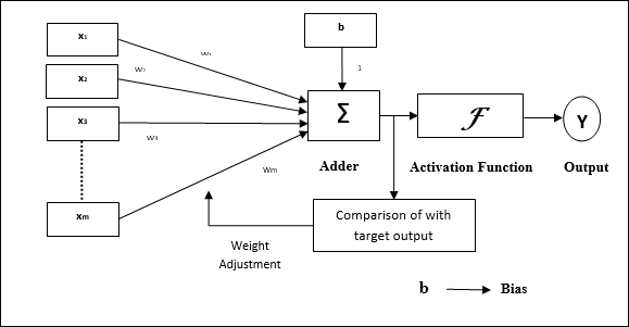
Fig 6: Adaline
Training Algorithm
The following is the Adaline network training algorithm:
Step 0: Set the weights and bias to some random numbers, but not zero. Set the parameter for learning rate.
Step 1: When the stopping condition is false, perform steps 2-6.
Step 2: for each bipolar training pair s:t, repeat steps 3-5.
Step 3: Set activations for input units i=1 to n.
Step 4: Calculate the net input to the output unit.
Step 5: For i=1 through n, update the weight and bias.
Step 6: Stop the training procedure if the maximum weight change during training is less than a defined tolerance, else continue. This is the test for a network's stopping condition.
Testing algorithm
It is critical to test a network after it has been taught. The Adaline can be used to classify input patterns once the training is complete. The network's performance is evaluated using a step function. The Adaline network's testing approach is as follows:
Step 1: Set up the weights. (The training algorithm determines the weights.)
Step 1: for each bipolar input vector x, repeat steps 2-4.
Step 2: set the input units' activations to x.
Step 3: Calculate the net input to the output units in step three.
Step 4: Apply the activation function to the derived net input.
Key takeaway
Adaline, which stands for Adaptive Linear Neuron, is a single-linear-unit network. It was created in 1960 by Widrow and Hoff.
More than one layer of artificial neurons or nodes makes up a multi-layer neural network. In terms of design, they are quite different. While single-layer neural networks were beneficial early in the creation of AI, today's networks almost all adopt a multi-layer approach.
There are a variety of approaches to set up multi-layer neural networks. They usually have at least one input layer that provides weighted inputs to a succession of hidden layers, followed by an output layer. Nonlinear designs employing sigmoids and other functions to direct the firing or activation of artificial neurons are also connected with these more advanced setups. While some of these systems are made of real materials, the majority are made of software functions that simulate cerebral activity.
Multi-layer neural networks include convolutional neural networks (CNNs), recurrent neural networks, deep networks, and deep belief systems, which are all useful for image processing and computer vision. CNNs, for example, can have dozens of layers working on an image in a sequential manner. Understanding how current neural networks work necessitates all of this.
Hidden layers, whose neurons are not directly connected to the output, are used in multilayer networks to address the classification issue for non-linear data. The hidden layers can be understood geometrically as additional hyper-planes that increase the network's separation capability. Typical multilayer network designs are depicted in Figure.
This new architecture raises a new challenge: how to train concealed units whose expected output is unknown. This problem can be solved using the Backpropagation technique.
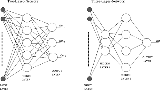
Fig 7: Example of multilayer neural network
The training is done in a supervised environment. The main principle is to feed the input vector into the network, then calculate the output of each layer and the network's final output in the forward direction. Because the target values for the output layer are known, the weights can be modified as if it were a single layer network; in the case of the BP method, using the gradient decent rule.
The mistake in the output layer is back-propagated to these layers according to the linking weights to determine the weight changes in the hidden layer. Each sample in the training set goes through the same procedure. An epoch is a single cycle across the training set. The number of epoches required to train the network is determined by a variety of factors, the most important of which is the error calculated in the output layer.
Key takeaway
More than one layer of artificial neurons or nodes makes up a multi-layer neural network. In terms of design, they are quite different. While single-layer neural networks were beneficial early in the creation of AI, today's networks almost all adopt a multi-layer approach.
The Backpropagation Algorithm is based on generalizing the Widrow-Hoff learning rule. It uses supervised learning, which means that the algorithm is provided with examples of the inputs and outputs that the network should compute, and then the error is calculated.
The backpropagation algorithm starts with random weights, and the goal is to adjust them to reduce this error until the ANN learns the training data.
Standard backpropagation is a gradient descent algorithm in which the network weights are moved along the negative of the gradient of the performance function.
The combination of weights that minimizes the error function is considered a solution to the learning problem.
The backpropagation algorithm requires a differentiable activation function, and the most commonly used are tan-sigmoid, log-sigmoid, and, occasionally, linear. Feed- forward networks often have one or more hidden layers of sigmoid neurons followed by an output layer of linear neurons. This structure allows the network to learn nonlinear and linear relationships between input and output vectors. The linear the output layer lets the network get values outside the range − 1 to + 1.
For the learning process, the data must be divided in two sets:
Training data set, which is used to calculate the error gradients and to update the weights; Validation data set, which allows selecting the optimum number of iterations to avoid overlearning.
As the number of iterations increases, the training error reduces whereas the validation data set error begins to drop, then reaches a minimum and finally increases. Continuing the learning process after the validation error arrives at a minimum leads to overlearning. Once the learning process is finished, another data set (test set) is used to validate and confirm the prediction accuracy.
Properly trained backpropagation networks tend to give reasonable answers when presented with new inputs. Usually, in ANN approaches, data normalization is necessary before starting the training process to ensure that the influence of the input variable in the course of model building is not biased by the magnitude of its native values, or its range of variation. The normalization technique, usually consists of a linear transformation of the input/output variables to the range (0, 1).
Feedforward Dynamics
When a Back Propagation network is cycled, the activations of the input units are propagated forward to the output layer through the connecting weights. As in perceptron, the net input to a unit is determined by the weighted sum of its inputs:
Netj = Σi wjiai
Where a i is the input activation from unit i and w ji is the weight connecting unit i to unit j. However, instead of calculating a binary output, the net input is added to the unit’s bias and the resulting value is passed through a sigmoid function:
The bias term plays the same role as the threshold in the perceptron. But unlike binary output of the perceptron, the output of a sigmoid is a continuous real-value between 0 and 1. The sigmoid function is sometimes called a”squashing” function because it maps its inputs onto a fixed range.
Convergence
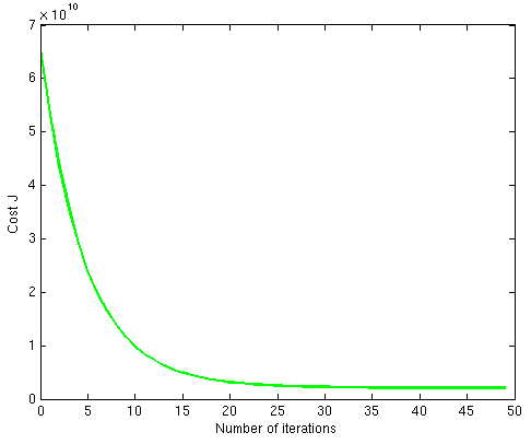
During training, a machine learning model reaches convergence when it reaches a state where it settles to within an error range around the final value. In other words, a model converges when it is no longer improved by more training.
Key takeaway
The Backpropagation Algorithm is based on generalizing the Widrow-Hoff learning rule.
The backpropagation algorithm starts with random weights, and the goal is to adjust them to reduce this error until the ANN learns the training data.
References:
- Tom Mitchell. Machine Learning (McGraw Hill)
- Understanding Machine Learning. Shai Shalev-Shwartz and Shai Ben-David. Cambridge University Press.
- Artificial Neural Network, B. Yegnanarayana, PHI, 2005