Unit - 3
Introduction to Trees
A tree is another data structure that can be used to represent hierarchical data. Nodes represent value and nodes are connected by edges.
Each node in the below structure is labeled with a number. Each arrow in the diagram below represents a link between the two nodes.

Fig 1: Tree
Root - In a tree hierarchy, the root node is the highest node. To put it another way, the root node is the one that has no children. The root node of the tree is numbered 1 in the above structure. A parent-child relationship exists when one node is directly linked to another node.
Child node - If a node is a descendant of another node, it is referred to as a child node.
Parent - If a node has a sub-node, the parent of that sub-node is said to be that node.
Sibling - Sibling nodes are those that have the same parent.
Leaf node - A leaf node is a node in the tree that does not have any descendant nodes. A leaf node is the tree's bottommost node. In a generic tree, there can be any number of leaf nodes. External nodes are also known as leaf nodes.
Internal node - An internal node is a node that has at least one child node.
Ancestor node - Any previous node on a path from the root to that node is an ancestor of that node. There are no ancestors for the root node. Nodes 1, 2, and 5 are the ancestors of node 10 in the tree depicted above.
Descendant node - A descendant of a node is the direct successor of the supplied node. In the diagram above, node 10 is a descendent of node 5.
Key takeaway
A tree is another data structure that can be used to represent hierarchical data. Nodes represent value and nodes are connected by edges.
The Binary tree means that the node can have a maximum of two children. Here, binary name itself suggests 'two'; therefore, each node can have either 0, 1 or 2 children.
Let's understand the binary tree through an example.
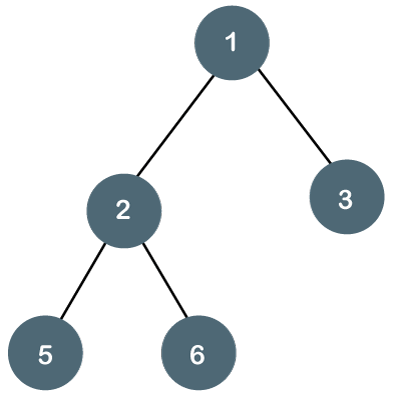
Fig 2: Example
The above tree is a binary tree because each node contains the utmost two children. The logical representation of the above tree is given below:
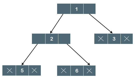
Fig 3: Logical representation
In the above tree, node 1 contains two pointers, i.e., left and a right pointer pointing to the left and right node respectively. The node 2 contains both the nodes (left and right node); therefore, it has two pointers (left and right). The nodes 3, 5 and 6 are the leaf nodes, so all these nodes contain NULL pointer on both left and right parts.
Properties of Binary Tree
● At each level of i, the maximum number of nodes is 2i.
● The height of the tree is defined as the longest path from the root node to the leaf node. The tree which is shown above has a height equal to 3. Therefore, the maximum number of nodes at height 3 is equal to (1+2+4+8) = 15. In general, the maximum number of nodes possible at height h is (20 + 21 + 22+….2h) = 2h+1 -1.
● The minimum number of nodes possible at height h is equal to h+1.
● If the number of nodes is minimum, then the height of the tree would be maximum. Conversely, if the number of nodes is maximum, then the height of the tree would be minimum.
If there are 'n' number of nodes in the binary tree.
The minimum height can be computed as:
As we know that,
n = 2h+1 -1
n+1 = 2h+1
Taking log on both the sides,
Log2(n+1) = log2(2h+1)
Log2(n+1) = h+1
h = log2(n+1) - 1
The maximum height can be computed as:
As we know that,
n = h+1
h= n-1
Types of Binary Tree
There are four types of Binary tree:
● Full/ proper/ strict Binary tree
● Complete Binary tree
● Perfect Binary tree
● Degenerate Binary tree
● Balanced Binary tree
Key takeaway
- The Binary tree means that the node can have a maximum of two children. Here, binary name itself suggests 'two'; therefore, each node can have either 0, 1 or 2 children.
Traversal is a process to visit all the nodes of a tree and may print their values too. Because all nodes are connected via edges (links) we always start from the root (head) node. That is, we cannot randomly access a node in a tree. There are three ways which we use to traverse a tree −
● In-order Traversal
● Pre-order Traversal
● Post-order Traversal
Generally, we traverse a tree to search or locate a given item or key in the tree or to print all the values it contains.
In-order Traversal
In this traversal method, the left subtree is visited first, then the root and later the right subtree. We should always remember that every node may represent a subtree itself.
If a binary tree is traversed in-order, the output will produce sorted key values in an ascending order.
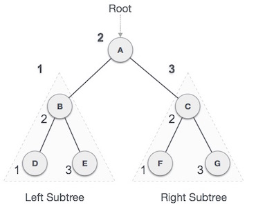
Fig 4: Inorder
We start from A, and following in-order traversal, we move to its left subtree B. B is also traversed in-order. The process goes on until all the nodes are visited. The output of inorder traversal of this tree will be −
D → B → E → A → F → C → G
Algorithm
Until all nodes are traversed −
Step 1 − Recursively traverse left subtree.
Step 2 − Visit root node.
Step 3 − Recursively traverse right subtree.
Pre-order Traversal
In this traversal method, the root node is visited first, then the left subtree and finally the right subtree.

Fig 5: Pre order
We start from A, and following pre-order traversal, we first visit A itself and then move to its left subtree B. B is also traversed pre-order. The process goes on until all the nodes are visited. The output of pre-order traversal of this tree will be −
A → B → D → E → C → F → G
Algorithm
Until all nodes are traversed −
Step 1 − Visit root node.
Step 2 − Recursively traverse left subtree.
Step 3 − Recursively traverse right subtree.
Post-order Traversal
In this traversal method, the root node is visited last, hence the name. First we traverse the left subtree, then the right subtree and finally the root node.
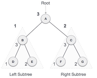
Fig 6: Post order
We start from A, and following Post-order traversal, we first visit the left subtree B. B is also traversed post-order. The process goes on until all the nodes are visited. The output of post-order traversal of this tree will be −
D → E → B → F → G → C → A
Algorithm
Until all nodes are traversed −
Step 1 − Recursively traverse left subtree.
Step 2 − Recursively traverse right subtree.
Step 3 − Visit root node.
A binary search tree is a type of binary tree in which the nodes are organized in a predetermined sequence. This is referred to as an ordered binary tree.
The value of all nodes in the left sub-tree is less than the value of the root in a binary search tree. Similarly, the value of all nodes in the right subtree is larger than or equal to the root's value. This rule will be applied recursively to all of the root's left and right subtrees.
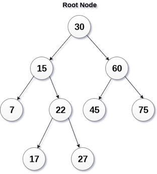
Fig 7: Binary search tree
A Binary Search Tree (BST) is a tree in which all nodes have the properties listed below.
● The key of the left subtree has a lower value than the key of its parent (root) node.
● The value of the right subkey tree's is larger than or equal to the value of the key of its parent (root) node.
● As a result, BST separates all of its sub-trees into two segments: the left and right subtrees, and can be characterized as
Left_subtree (keys) < node (key) ≤ right_subtree (keys)
Insertion
The insertion operation in a binary search tree takes O(log n) time to complete. A new node is always added as a leaf node in a binary search tree. The following is how the insertion procedure is carried out.
Step 1: Create a newNode with the specified value and NULL left and right.
Step 2: Make sure the tree isn't empty.
Step 3 - Set root to newNode if the tree is empty.
Step 4 - If the tree isn't empty, see if newNode's value is smaller or larger than the node's value (here it is root node).
Step 5 - Go to the node's left child if newNode is smaller or equal to it. Move to new Nodes right child if the newNode is larger than the node.
Step 6- Continue in this manner until we reach the leaf node (i.e., reaches to NULL).
Step 7 - Once you've reached the leaf node, insert the newNode as a left child if it's smaller or equal to the leaf node, or as a right child otherwise.
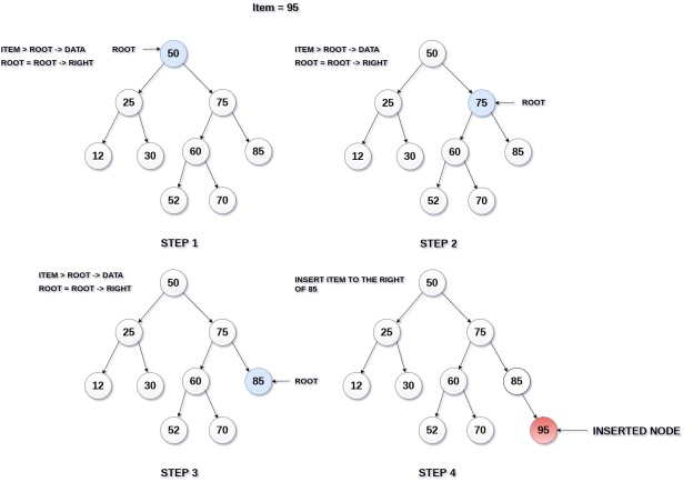
Fig 8: Example of insertion
Deletion
The deletion process in a binary search tree takes O(log n) time to complete. The three scenarios for removing a node from a Binary search tree are as follows.
Case 1: Deleting a Leaf node (A node with no children)
Case 2: Deleting a node with one child
Case 3: Deleting a node with two children
Case 1: Deleting a Leaf node
To delete a leaf node from BST, follow these steps...
Step 1: Using the search function, locate the node to be eliminated.
Step 2 - If the node is a leaf, delete it with the free function and end the function.
Case 2: Deleting a node with one child
To delete a node with one child from BST, we utilize the procedures below...
Step 1: Using the search function, locate the node to be eliminated.
Step 2 - Create a link between the parent node and the child node if it only has one child.
Step 3: Using the free function, delete the node and exit the function
Case 3: Deleting a node with two children
To delete a node with two children from BST, we utilize the procedures below...
Step 1: Using the search function, locate the node to be eliminated.
Step 2 - Find the largest node in the left subtree (OR the smallest node in the right subtree) if it has two children.
Step 3 - Swap the deleting node with the node discovered in the previous step.
Step 4 - Next, see if deleting the node resulted in case 1 or case 2, if not, move to step 2.
Step 5 - If case 1 applies, delete it using case 1 reasoning.
Step 6- If case 2 applies, delete it using case 2 reasoning.
Step 7 - Continue in this manner until the node has been removed from the tree.
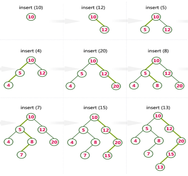
Example
Create a Binary Search Tree by adding the integers in the following order.
10,12,5,4,20,8,7,15 and 13
The following items are added into a Binary Search Tree in the following order.
Key takeaway
A binary search tree is a type of binary tree in which the nodes are organized in a predetermined sequence.
This is referred to as an ordered binary tree.
When only one thread is used in a threaded binary tree, it is referred to as a one way threaded tree, and when both threads are used, it is referred to as a two way threaded tree. When the pointer is set to the root node, If neither an in-order predecessor nor an in-order successor can be found.
Here we will see the threaded binary tree data structure. We know that the binary tree nodes may have at most two children. But if they have only one child, or no children, the link part in the linked list representation remains null. Using threaded binary tree representation, we can reuse that empty link by making some threads.
If one node has some vacant left or right child area, that will be used as thread. There are two types of threaded binary tree. The single threaded tree or fully threaded binary tree. In single threaded mode, there are another two variations. Left threaded and right threaded.
In the left threaded mode if some node has no left child, then the left pointer will point to its inorder predecessor, similarly in the right threaded mode if some node has no right child, then the right pointer will point to its inorder successor. In both cases, if no successor or predecessor is present, then it will point to the header node.
For fully threaded binary tree, each node has five fields. Three fields like normal binary tree node, another two fields to store Boolean value to denote whether link of that side is actual link or thread.
One way threaded tree
● A node's empty left child field can be used to reference its inorder predecessor.
● In the same way, a node's empty right child field can be used to point to its in-order successor.
● A one-way threaded binary tree is one such form of binary tree.
● Thread is a field that stores the address of its in-order successor.
A single-threaded tree is also known as a one-way threaded tree. If the thread is found in the left field, the left field will be changed to point to the node's in-order predecessor. A left-threaded binary tree is a one-way threaded tree with only one direction of threading.
Example
A binary tree with one-way threading and its linked form are shown in the diagram.
Because node5's RIGHT field has a NULL pointer, it will be replaced to point to node1, which is its in-order successor. Similarly, node 8's RIGHT field will point to node 4, node 9's RIGHT field will point to node 2, node 10's RIGHT field will point to node 6, node 11's RIGHT field will point to node 3, and node 12's RIGHT field will contain NULL because it has no in order successor.
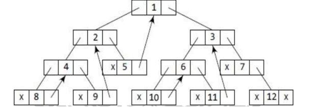
Fig 9: One way threaded tree
Two way binary threaded tree
● A threaded binary tree is one example of this sort of binary tree.
● Thread is a field that stores the address of its inorder successor or predecessor.
● A node's empty left child field can be used to reference its inorder predecessor.
● In the same way, a node's empty right child field can be used to point to its inorder successor.
Figure shows a binary tree without threading and its corresponding linked representation.
The in-order traversal of the tree is given as 8, 4, 9, 2, 5, 1, 10, 6, 11,3, 7, 12
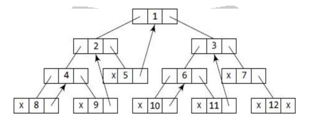
Fig 10: Two way binary tree
Key takeaway
- Here we will see the threaded binary tree data structure. We know that the binary tree nodes may have at most two children.
- But if they have only one children, or no children, the link part in the linked list representation remains null.
- Using threaded binary tree representation, we can reuse that empty links by making some threads.
AVL Tree was invented by GM Adelson - Velsky and EM Landis in 1962. The tree is named AVL in honour of its inventors.
AVL Tree can be defined as a height balanced binary search tree in which each node is associated with a balance factor which is calculated by subtracting the height of its right subtree from that of its left sub-tree.
Tree is said to be balanced if the balance factor of each node is in between -1 to 1, otherwise, the tree will be unbalanced and need to be balanced.
Balance Factor (k) = height (left(k)) - height (right(k))
If balance factor of any node is 1, it means that the left sub-tree is one level higher than the right subtree.
If balance factor of any node is 0, it means that the left subtree and right subtree contain equal height.
If balance factor of any node is -1, it means that the left sub-tree is one level lower than the right subtree.
An AVL tree is given in the following figure. We can see that, balance factor associated with each node is in between -1 and +1. Therefore, it is an example of AVL tree.
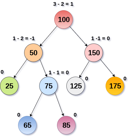
Fig 11: AVL Tree
Complexity
Algorithm | Average case | Worst case |
Space | o(n) | o(n) |
Search | o(log n) | o(log n) |
Insert | o(log n) | o(log n) |
Delete | o(log n) | o(log n) |
Operations on AVL tree
Due to the fact that, AVL tree is also a binary search tree therefore, all the operations are performed in the same way as they are performed in a binary search tree. Searching and traversing do not lead to the violation in property of AVL tree. However, insertion and deletion are the operations which can violate this property and therefore, they need to be revisited.
SN | Operation | Description |
1 | Insertion | Insertion in AVL tree is performed in the same way as it is performed in a binary search tree. However, it may lead to violation in the AVL tree property and therefore the tree may need balancing. The tree can be balanced by applying rotations. |
2 | Deletion | Deletion can also be performed in the same way as it is performed in a binary search tree. Deletion may also disturb the balance of the tree therefore, various types of rotations are used to rebalance the tree. |
Why AVL Tree?
AVL tree controls the height of the binary search tree by not letting it to be skewed. The time taken for all operations in a binary search tree of height h is O(h). However, it can be extended to O(n) if the BST becomes skewed (i.e. worst case). By limiting this height to log n, AVL tree imposes an upper bound on each operation to be O(log n) where n is the number of nodes.
AVL Rotations
We perform rotation in AVL tree only in case if Balance Factor is other than -1, 0, and 1. There are basically four types of rotations which are as follows:
- L L rotation: Inserted node is in the left subtree of left subtree of A
- R R rotation: Inserted node is in the right subtree of right subtree of A
- L R rotation: Inserted node is in the right subtree of left subtree of A
- R L rotation: Inserted node is in the left subtree of right subtree of A
Where node A is the node whose balance Factor is other than -1, 0, 1.
The first two rotations LL and RR are single rotations and the next two rotations LR and RL are double rotations. For a tree to be unbalanced, minimum height must be at least 2, Let us understand each rotation
1. RR Rotation
When BST becomes unbalanced, due to a node is inserted into the right subtree of the right subtree of A, then we perform RR rotation, RR rotation is an anticlockwise rotation, which is applied on the edge below a node having balance factor -2
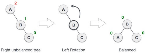
Fig 12: RR rotation
In above example, node A has balance factor -2 because a node C is inserted in the right subtree of A right subtree. We perform the RR rotation on the edge below A.
2. LL Rotation
When BST becomes unbalanced, due to a node is inserted into the left subtree of the left subtree of C, then we perform LL rotation, LL rotation is clockwise rotation, which is applied on the edge below a node having balance factor 2.

Fig 13: LL rotations
In above example, node C has balance factor 2 because a node A is inserted in the left subtree of C left subtree. We perform the LL rotation on the edge below A.
3. LR Rotation
Double rotations are bit tougher than single rotation which has already explained above. LR rotation = RR rotation + LL rotation, i.e., first RR rotation is performed on subtree and then LL rotation is performed on full tree, by full tree we mean the first node from the path of inserted node whose balance factor is other than -1, 0, or 1.
Let us understand each and every step very clearly:
State | Action |
 | A node B has been inserted into the right subtree of A the left subtree of C, because of which C has become an unbalanced node having balance factor 2. This case is L R rotation where: Inserted node is in the right subtree of left subtree of C |
 | As LR rotation = RR + LL rotation, hence RR (anticlockwise) on subtree rooted at A is performed first. By doing RR rotation, node A, has become the left subtree of B. |
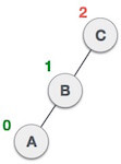 | After performing RR rotation, node C is still unbalanced, i.e., having balance factor 2, as inserted node A is in the left of left of C |
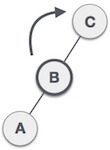 | Now we perform LL clockwise rotation on full tree, i.e. on node C. Node C has now become the right subtree of node B, A is left subtree of B |
 | Balance factor of each node is now either -1, 0, or 1, i.e. BST is balanced now. |
4. RL Rotation
As already discussed, that double rotations are bit tougher than single rotation which has already explained above. R L rotation = LL rotation + RR rotation, i.e., first LL rotation is performed on subtree and then RR rotation is performed on full tree, by full tree we mean the first node from the path of inserted node whose balance factor is other than -1, 0, or 1.
State | Action |
 | A node B has been inserted into the left subtree of C the right subtree of A, because of which A has become an unbalanced node having balance factor - 2. This case is RL rotation where: Inserted node is in the left subtree of right subtree of A |
 | As RL rotation = LL rotation + RR rotation, hence, LL (clockwise) on subtree rooted at C is performed first. By doing RR rotation, node C has become the right subtree of B. |
 | After performing LL rotation, node A is still unbalanced, i.e. having balance factor -2, which is because of the right-subtree of the right-subtree node A. |
 | Now we perform RR rotation (anticlockwise rotation) on full tree, i.e. on node A. Node C has now become the right subtree of node B, and node A has become the left subtree of B. |
 | Balance factor of each node is now either -1, 0, or 1, i.e., BST is balanced now. |
Q: Construct an AVL tree having the following elements
H, I, J, B, A, E, C, F, D, G, K, L
1. Insert H, I, J
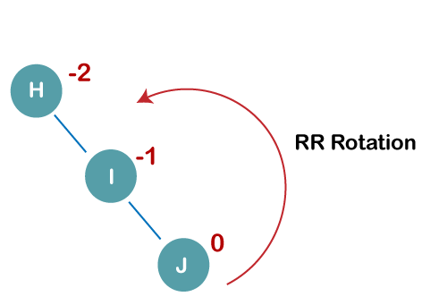
On inserting the above elements, especially in the case of H, the BST becomes unbalanced as the Balance Factor of H is -2. Since the BST is right-skewed, we will perform RR Rotation on node H.
The resultant balance tree is:

2. Insert B, A
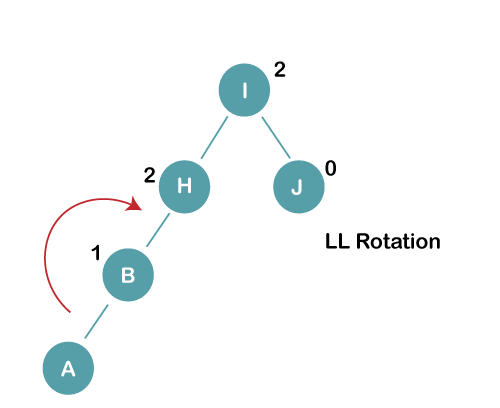
On inserting the above elements, especially in case of A, the BST becomes unbalanced as the Balance Factor of H and I is 2, we consider the first node from the last inserted node i.e. H. Since the BST from H is left-skewed, we will perform LL Rotation on node H.
The resultant balance tree is:
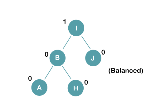
3. Insert E
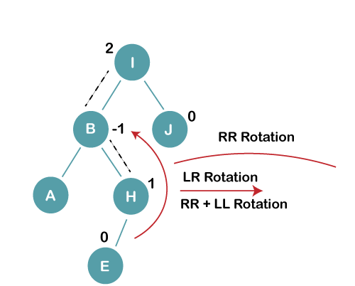
On inserting E, BST becomes unbalanced as the Balance Factor of I is 2, since if we travel from E to I we find that it is inserted in the left subtree of right subtree of I, we will perform LR Rotation on node I. LR = RR + LL rotation
3 a) We first perform RR rotation on node B
The resultant tree after RR rotation is:
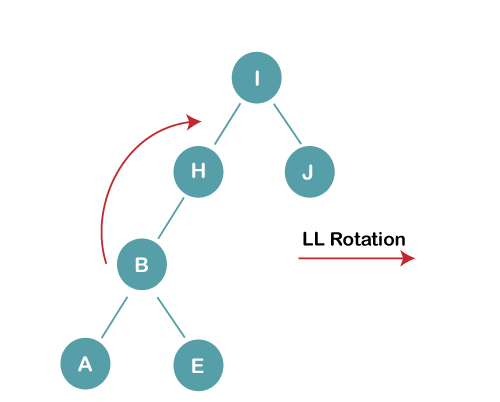
3b) We first perform LL rotation on the node I
The resultant balanced tree after LL rotation is:
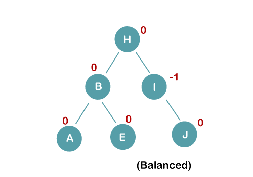
4. Insert C, F, D
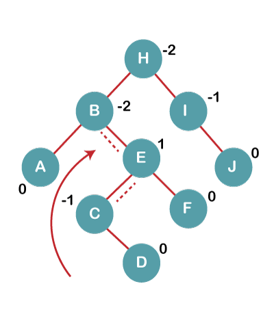
On inserting C, F, D, BST becomes unbalanced as the Balance Factor of B and H is -2, since if we travel from D to B we find that it is inserted in the right subtree of left subtree of B, we will perform RL Rotation on node I. RL = LL + RR rotation.
4a) We first perform LL rotation on node E
The resultant tree after LL rotation is:
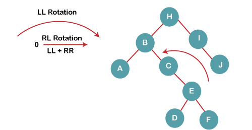
4b) We then perform RR rotation on node B
The resultant balanced tree after RR rotation is:
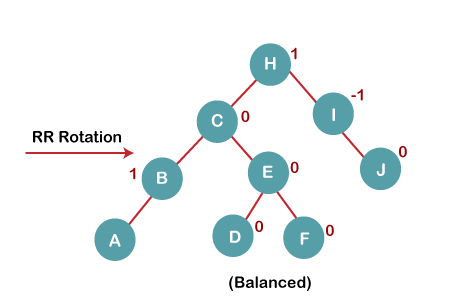
5. Insert G
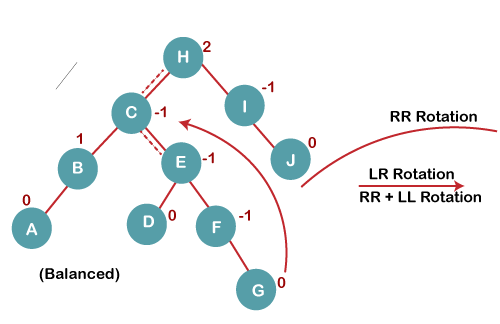
On inserting G, BST become unbalanced as the Balance Factor of H is 2, since if we travel from G to H, we find that it is inserted in the left subtree of right subtree of H, we will perform LR Rotation on node I. LR = RR + LL rotation.
5 a) We first perform RR rotation on node C
The resultant tree after RR rotation is:
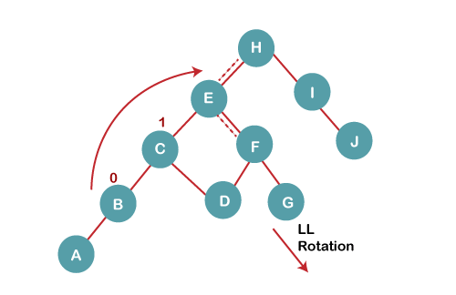
5 b) We then perform LL rotation on node H
The resultant balanced tree after LL rotation is:
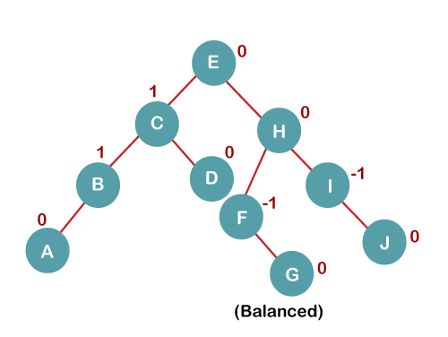
6. Insert K

On inserting K, BST becomes unbalanced as the Balance Factor of I is -2. Since the BST is right-skewed from I to K, hence we will perform RR Rotation on the node I.
The resultant balanced tree after RR rotation is:
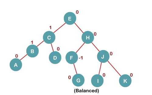
7. Insert L
On inserting the L tree is still balanced as the Balance Factor of each node is now either, -1, 0, +1. Hence the tree is a Balanced AVL tree

Key takeaway
- AVL Tree was invented by GM Adelson - Velsky and EM Landis in 1962. The tree is named AVL in honour of its inventors.
- AVL Tree can be defined as height balanced binary search tree in which each node is associated with a balance factor which is calculated by subtracting the height of its right subtree from that of its left sub-tree.
- Tree is said to be balanced if balance factor of each node is in between -1 to 1, otherwise, the tree will be unbalanced and need to be balanced.
An extended binary tree is a sort of binary tree in which all of the original tree's null subtrees are replaced with special nodes known as external nodes, while other nodes are known as internal nodes.
The internal nodes are represented by circles, whereas the external nodes are represented by boxes.
- Internal nodes are those from the original tree, whereas external nodes are those from the special tree.
- Internal nodes are non-leaf nodes, while all external nodes are leaf nodes.
- Every exterior node is a leaf, and every internal node has precisely two children.
- It shows the outcome, which is a full binary tree.
It is not required that all nodes have the same number of children, but each node must include m/2 nodes.
The following graphic depicts a B tree of order 4.

Fig 14: B tree
Any attribute of B Tree may be violated while performing some operations on it, such as the number of minimum children a node can have. The tree may split or unite in order to keep the features of B Tree.
Application of B tree
Because accessing values held in a huge database that is saved on a disk is a very time consuming activity, B tree is used to index the data and enable fast access to the actual data stored on the disks.
In the worst situation, searching an unindexed and unsorted database with n key values takes O(n) time. In the worst-case scenario, if we use B Tree to index this database, it will be searched in O(log n) time.
Operations
Searching
B Trees are comparable to Binary Search Trees in terms of searching. For example, let's look for item 49 in the B Tree below. The procedure will go somewhat like this:
- Compare item 49 to node 78, which is the root node. Move to the left sub-tree since 49 78 onwards.
- Since 404956, move to the right subtree of 40. 49>45, move to the right subtree of 40.
- Compare and contrast 49.
- Return if a match is found.
The height of the tree affects the search in a B tree. To search any element in a B tree, the search technique requires O(log n) time.

Inserting
At the leaf node level, insertions are made. In order to place an item into B Tree, the following algorithm must be followed.
- Navigate the B Tree until you find the suitable leaf node to insert the node at.
- If there are fewer than m-1 keys in the leaf node, insert the element in ascending order.
- Otherwise, if the leaf node contains m-1 keys, proceed to the next step.
● In the rising sequence of elements, add the new element.
● At the middle, divide the node into two nodes.
● The median element should be pushed up to its parent node.
● If the parent node has the same m-1 number of keys as the child node, split it as well.
Deletion
At the leaf nodes, deletion is also conducted. It can be a leaf node or an inside node that needs to be destroyed. In order to delete a node from a B tree, use the following algorithm.
- Locate the leaf node.
- If the leaf node has more than m/2 keys, delete the required key from the node.
- If the leaf node lacks m/2 keys, fill in the gaps with the element from the eighth or left sibling.
● If the left sibling has more than m/2 elements, shift the intervening element down to the node where the key is deleted and push the largest element up to its parent.
● If the right sibling has more than m/2 items, shift the intervening element down to the node where the key is deleted and push the smallest element up to the parent.
4. Create a new leaf node by merging two leaf nodes and the parent node's intervening element if neither sibling has more than m/2 elements. If the parent has less than m/2 nodes, repeat the operation on the parent as well.
5. If the node to be destroyed is an internal node, its in-order successor or predecessor should be used instead. The process will be same as the node is deleted from the leaf node because the successor or predecessor will always be on the leaf node.
Key takeaway
An extended binary tree is a sort of binary tree in which all of the original tree's null subtrees are replaced with special nodes known as external nodes, while other nodes are known as internal nodes.
References:
- Data Structures and Algorithms in C, M.T. Goodrich, R. Tamassia and D. Mount, Wiley India.
- Data Structures Using C – A.M. Tenenbaum (PHI)
- Data Structures and Algorithm Analysis in C, 3rd Edition, M.A. Weiss, Pearson.
- Classic Data Structures, D. Samanta, 2nd Edition, PHI.
- Data Structure Using C by Pankaj Kumar Pandey.