Unit - 4
Image Restoration and Segmentation
Image restoration is the operation of taking a corrupt/noisy image and estimating the clean, original image. Corruption may come in many forms such as motion blur, noise, and camera misfocus. Image restoration is performed by reversing the process that blurred the image and such is performed by imaging a point source and use the point source image, which is called the Point Spread Function (PSF) to restore the image information lost to the blurring process.
Image restoration is different from image enhancement in that the latter is designed to emphasize features of the image that make the image more pleasing to the observer, but not necessarily to produce realistic data from a scientific point of view. Image enhancement techniques (like contrast stretching or de-blurring by the nearest neighbour procedure) provided by imaging packages use no a priori model of the process that created the image.
With image, enhancement noise can effectively be removed by sacrificing some resolution, but this is not acceptable in many applications. In a fluorescence microscope, the resolution in the z-direction as bad as it is. More advanced image processing techniques must be applied to recover the object.
The objective of image restoration techniques is to reduce noise and recover resolution loss Image processing techniques are performed either in the image domain or the frequency domain. The most straightforward and conventional technique for image restoration is deconvolution, which is performed in the frequency domain and after computing the Fourier transform of both the image and the PSF and undo the resolution loss caused by the blurring factors. This deconvolution technique, because of its direct inversion of the PSF which typically has poor matrix condition number, amplifies noise and creates an imperfect deblurred image. Also, conventionally the blurring process is assumed to be shift-invariant. Hence more sophisticated techniques, such as regularized deblurring, have been developed to offer robust recovery under different types of noises and blurring functions. It is of 3 types: 1. Geometric correction 2. Radiometric correction 3. Noise removal
A model for the Image Degradation/Restoration process

g(x, y) = h(x, y) * f(x, y) + η(x, y)
G (u, v) = H (u, v) F (u, v) + N (u, v)
Noise Models
Gaussian Noise
Mathematically tractable in both spatial and frequency domain. PDF of a Gaussian random variable z is given by
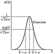
z = Intensity
z = Mean (average)
σ = Standard deviation
σ2 = Variance of z
p(z) = 1/√2𝝅σ×e -(z-z)2/ 2σ2
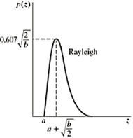
Rayleigh Noise
Displacement from origin
Skewed to the right
Erlang(gamma) noise

Mean z = a +√𝝅b/4
Variance σ2 = b(4-𝝅)/4
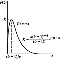
Pdf of Erlang Noise is p(z) =
Where a>0 and b is positive integer
Mean z = b/a and variance σ2 = b/a2
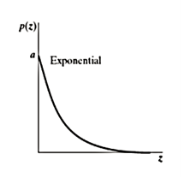
Exponential noise
The pdf of this noise is
P(z) = ae-az for z≥0
0 for z< 0
Where a>0
Mean z = 1/a andvariance σ2 = 1/ a2
This is a special case of Erlang Noise with b=1
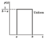
Uniform Noise
PDF of uniform noise is given by

Mean = z =a+b/2
Variance = σ2 = (b-a)2/12
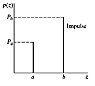
Impulse (Salt and Pepper Noise)
PDF of impulse noise is

If b>a, intensity b will appear as alight dot in the image a will appear as dark dot
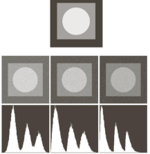
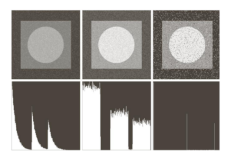
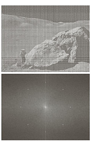
Periodic Noise
Restoration in the presence of noise only-Spatial filtering
g(x, y) = f(x, y) + n(x, y ) and
G(u, v) = F(u, v) + N(u, v)
Key takeaway
Image restoration is the operation of taking a corrupt/noisy image and estimating the clean, original image. Corruption may come in many forms such as motion blur, noise, and camera misfocus. Image restoration is performed by reversing the process that blurred the image and such is performed by imaging a point source and use the point source image, which is called the Point Spread Function (PSF) to restore the image information lost to the blurring process.
Mean Filters
In this section, we discuss briefly the noise-reduction spatial filters introduced in Section 3.6 and develop several other filters whose performance is in many cases superior to the filters discussed in that section.
Arithmetic mean filter
This is the simplest of the mean filters. Let Sxv represent the set of coordinates in a rectangular sub-image window of size m X n, centered at the point (x, y).The arithmetic means filtering process computes the average value of the corrupted image g (x, y) in the area defined by Sxy.The value of the restored image at any point (x, y) is simply the arithmetic mean computed using the pixels in the region defined by S. In other words.
fᵔ (x, y) = 1/mn ∑ (s.t) S xy g (s, t )
This operation can be implemented using a convolution mask in which ail coefficients have a value of 1/mn. As discussed in Section 3.6.1, a mean filter simply smoothes local variations in an image. Noise is reduced as a result of blurring.
Geometric mean filter
An image restored using a geometric mean filter is given by the expression
fᵔ (x, y) = π(s.t) ᵋ S xy g(s, t) 1/mn
Here, each restored pixel is given by the product of the pixels in the sub-image window, raised to the power 1/mn. As shown in Example 52, a geometric mean filter achieves smoothing comparable to the arithmetic mean filter, but it tends to lose less image detail in the process.
Harmonic mean filter
The harmonic mean filtering operation is given by the expression
fᵔ (x, y) = mn / ∑ (s.t) ᵋ S xy 1/ g (s, t )
The harmonic mean filter works well for salt noise but fails for pepper noise. It does well also with other types of noise like Gaussian noise.
Contraharmonic mean filter
The contraharmonic mean filtering operation yields a restored image based on the expression

Where Q is called the order of the filter. This filter is well suited for reducing or virtually eliminating the effects of salt-and-pepper noise. For positive values of Q, the filter eliminates pepper noise. For negative values of Q, it eliminates salt noise. It cannot do both simultaneously. Note that the contraharmonic filter reduces to the arithmetic mean filter if Q = 0, and to the harmonic mean filter if Q = - 1
Order-Statistics Filters
Order-statistics filters were introduced in Section 3.6.2. We now expand the discussion in that section and introduce some additional order-statistics filters. As noted in Section 3.6.2, order-statistics filters are spatial filters whose response is based on ordering (ranking) the pixels contained in the image area encompassed by the filter. The response of the filter at any point is determined by the ranking result
Median filter
The best-known order-statistics filter is the median filter, which, as its name implies, replaces the value of a pixel by the median of the gray levels in the neighborhood of that pixel:
F(x, y) = median(s, y)*Sxy {g(s, t)}
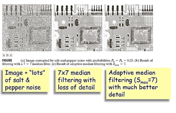
The original value of the pixel is included in the computation of the median. Median filters are quite popular because, for certain types of random noise, they provide excellent noise-reduction capabilities, with considerably less blurring than linear smoothing filters of similar size. Median filters are particularly effective in the presence of both bipolar and unipolar impulse noise. In fact, as Example 5.3 shows, the median filter yields excellent results for images corrupted by this type of noise.
Max and min filters
Although the median filter is by far the order-statistics filter most used in image processing.it is by no means the only one. The median represents the 50th percentile of a ranked set of numbers, but the reader will recall from basic statistics that ranking lends itself to many other possibilities. For example, using the 100th percentile results in the so-called max filter given by:
f(x, y) = max(s, t)*Sxy {g(s, t)}
This filter is useful for finding the brightest points in an image. Also, because pepper noise has very low values, it is reduced by this filter as a result of the max selection process in the sub-image area S. The 0th percentile filter is the Min filter.
f(x, y) = min(s, t)*Sxy {g(s, t)}
Key takeaway
This is the simplest of the mean filters. Let Sxv represent the set of coordinates in a rectangular sub-image window of size m X n, centered at the point (x, y).The arithmetic means filtering process computes the average value of the corrupted image g (x, y) in the area defined by Sxy.The value of the restored image at any point (x, y) is simply the arithmetic mean computed using the pixels in the region defined by S.
fᵔ (x, y) = g (x, y) - σ2n / σ2L [g (x, y) – mL]
σ2n Noise variance over the entire image (estimated)
mL Local mean (calculated)
σ2n Local variance (calculated)
DIFFERENT CASES
- If σ2n = σ2L the filter returns the local mean thus averaging out the noise
- If σ2n<<σ2L this is probably the location of an edge and we should return the edge value, i.e., g(x, y)
- If σ2n = 0 there is no noise and we return g(x, y)
- If σ2n>σ2L we can get negative gray scale values which is a potential problem
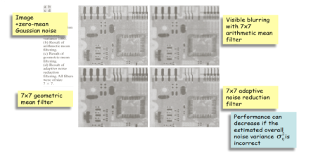
Varies Sxy to reduce impulsive noise
Stage A: IF zmed>Zmin and Zmax>Zmed
THEN go to Stage B
ELSE increase the window size Sxy
IF WindowSize≤ Smax
THEN goto Level A
Stage B: IF zxy>zminandzmax>zxy
THEN output zxy
ELSE output zmed
Zminmin. Gray value in Sxy
Zmaxmax. Gray value in Sxy
Zmedmedian gray value inSxy
Zxy gray level valueat (x, y)
Smax max. Allowed size of Sxy
If zmax>zmed>zmin thenzmed is NOT an impulse and we go to Stage B. Otherwise Stage A continues to increase the neighborhood Sxy until zmed is not an impulse.
If zmax>zxy>zminthenzxy is NOT an impulse and we output zxyotherwise we output the median zmed.
The fundamental idea is to increase the size of the neighbourhoodSxy until we are sufficiently sure that zxy is impulsive or not. If it is impulsive then output the median otherwise output zxy.
The BANDREJECT_FILTER function applies a low-reject, high-reject, or band-reject filter on a one-channel image.
A band-reject filter is useful when the general location of the noise in the frequency domain is known. A band-reject filter blocks frequencies within the chosen range and lets frequencies outside of the range pass through.
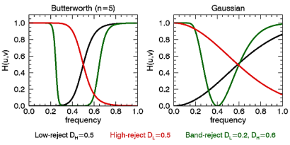
The following diagrams give a visual interpretation of the transfer functions:
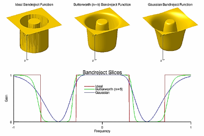
Fig – Band reject
This routine is written in the IDL language. Its source code can be found in the file bandreject_filter.pro in the lib subdirectory of the IDL distribution.
Syntax
Result = BANDREJECT_FILTER (ImageData, LowFreq, HighFreq [, /IDEAL] [, BUTTERWORTH=value] [, /GAUSSIAN])
Return Value
Returns a filtered image array of the same dimensions and type as ImageData.
Arguments
ImageData
A two-dimensional array containing the pixel values of the input image.
LowFreq
The lower limit of the cut-off frequency band. This value should be between 0 and 1 (inclusive) and must be less than HighFreq.
HighFreq
The upper limit of the cut-off frequency band. This value should be between 0 and 1 (inclusive) and must be greater than LowFreq.
Keywords
IDEAL
Set this keyword to use an ideal band-reject filter. In this type of filter, frequencies outside of the given range are passed without attenuation, and frequencies inside of the given range are blocked. This behavior makes the ideal band-reject filters very sharp.
The centered Fast Fourier Transform (FFT) is filtered by the following function, where DL is the lower bound of the frequency band, DH is the upper bound of the frequency band, and D (u, v) is the distance between a point (u, v) in the frequency domain and the center of the frequency rectangle:

BUTTERWORTH
Set this keyword to the dimension of the Butterworth filter to apply to the frequency domain. With a Butterworth band-reject filter, frequencies at the center of the frequency band are completely blocked and frequencies at the edge of the band are attenuated by a fraction of the maximum value. The Butterworth filter does not have any sharp discontinuities between passed and filtered frequencies.
Note: The default for BANDREJECT_FILTER is BUTTERWORTH=1.
The centered FFT is filtered by one of the following functions, where D0 is the center of the frequency
Low-reject (DL = 0, DH < 1):H (u, v) = 1 – 1/ 1+[D/DH]2n
Band -reject (DL > 0, DH < 1):H (u, v) = 1/ 1+[(DW)/ (D2- D20]2n
High- reject (DL > 0, DH = 1):H (u, v) = 1 – 1/ 1+ [DL / D]2n
Cy band, W is the width of the frequency band, D=D (u, v) is the distance between a point (u, v) in the frequency domain and the center of the frequency rectangle, and n is the dimension of the Butterworth filter:
Note: A low Butterworth dimension is close to Gaussian, and a high Butterworth dimension is close to Ideal.
GAUSSIAN
Set this keyword to use a Gaussian band-reject filter. In this type of filter, the transition between unfiltered and filtered frequencies is very smooth.
The centered FFT is filtered by one of the following functions, where D0 is the center of the frequency band, W is the width of the frequency band, and D=D (u, v) is the distance between a point (u, v) in the frequency domain and the center of the frequency rectangle:
Examples
Here, we plot the frequency response of the Butterworth (n=5) and Gaussian filters. For the low-reject filter we use a high-frequency cut-off of 0.5, for high-reject we use a cut-off of 0.5, and for the band-reject we use DL=0.2 and DH=0.6.
m = [0.2,0.27,0.05,0.1]
p = PLOT('1-1/(1 + (X/0.5)^10)', '3', DIM=[600,300], FONT_SIZE=10, $
XRANGE=[0,1], YRANGE=[0,1.1], LAYOUT=[2,1,1], MARGIN=m, $
XTITLE='frequency', YTITLE='H(u,v)', TITLE='Butterworth (n=5)')
p = PLOT('1/(1 + (X*0.4/(X^2-0.4^2))^10)', '3g', /OVERPLOT)
p = PLOT('1-1/(1 + (0.5/X)^10)', '3r', /OVERPLOT)
p = PLOT('1-exp(-X^2/(2*0.5^2))', '3', DIM=[600,300], FONT_SIZE=10, $
XRANGE=[0,1], YRANGE=[0,1.1], LAYOUT=[2,1,2], MARGIN=m, $
XTITLE='frequency', YTITLE='H(u,v)', TITLE='Gaussian', /CURRENT)
p = PLOT('1-exp(-((X^2-0.4^2)/(X*0.4))^2)', '3g', /OVERPLOT)
p = PLOT('exp(-X^2/(2*0.5^2))', '3r', /OVERPLOT)
t = TEXT(0.12,0.05,'Low-reject $D_H=0.5$',/NORM, FONT_SIZE=9)
t = TEXT(0.38,0.05,'High-reject $D_L=0.5$',COLOR='red',/NORM, FONT_SIZE=9)
t = TEXT(0.64,0.05,'Band-reject $D_L=0.2, D_H=0.6$', $
COLOR='green',/NORM, FONT_SIZE=9)
p.Save, 'bandreject_filter.png', resolution=120
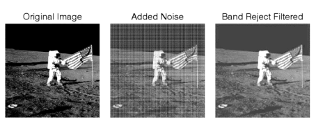
In the following example, we add some sinusoidal noise to an image and filter it with BANDREJECT_FILTER.
; Read in the file
File = FILEPATH('moon_landing.png', SUBDIR=['examples','data'])
ImageOriginal = READ PNG(file)
; Generate some sinusoidal noise
XCoords = LINDGEN(300,300) MOD 300
YCoords = TRANSPOSE(xCoords)
Noise = -SIN(xCoords*1.5)-SIN(yCoords*1.5)
ImageNoise = imageOriginal + 50*noise
; Filter the noise with a band reject filter
ImageFiltered = BRANDREJECT FILTER(imageNoise, 0.28, 0.38)
; Display the original, noise-added, and filtered images
i=IMAGE(imageOriginal, LAYOUT=[3,1,1], TITLE='Original Image', $
DIMENSIONS=[700,300])
i=IMAGE(imageNoise, LAYOUT=[3,1,2], /CURRENT, TITLE='Added Noise')
i=IMAGE(imageFiltered, LAYOUT=[3,1,3], /CURRENT, $
TITLE='Band Reject Filtered')
i.Save, 'bandreject_filter_ex.gif', resolution=120
Key takeaway
The BANDREJECT_FILTER function applies a low-reject, high-reject, or band-reject filter on a one-channel image.
A band-reject filter is useful when the general location of the noise in the frequency domain is known. A band-reject filter blocks frequencies within the chosen range and lets frequencies outside of the range pass through.
The BANDPASS_FILTER function applies a lowpass, bandpass, or highpass filter to a one-channel image.
A bandpass filter is useful when the general location of the noise in the frequency domain is known. The bandpass filter allows frequencies within the chosen range through and attenuates frequencies outside of the given range.
The following diagrams give a visual interpretation of the transfer functions:
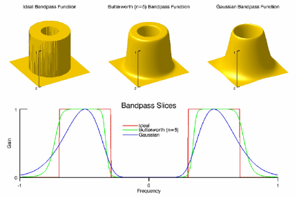
Fig – Bandpass
This routine is written in the IDL language. Its source code can be found in the file bandpass_filter.pro in the lib subdirectory of the IDL distribution.
Syntax
Result = BANDPASS_FILTER( ImageData, LowFreq, HighFreq [, /IDEAL] [, BUTTERWORTH=value] [, /GAUSSIAN] )
Return Value
Returns a filtered image array of the same dimensions and type as ImageData.
Arguments
ImageData
A two-dimensional array containing the pixel values of the input image.
LowFreq
The lower limit of the pass-through frequency band. This value should be between 0 and 1 (inclusive) and must be less than HighFreq.
HighFreq
The upper limit of the pass-through frequency band. This value should be between 0 and 1 (inclusive) and must be greater than LowFreq.
Keywords
IDEAL
Set this keyword to use an ideal bandpass filter. Ideal bandpass filters, frequencies within the given range are passed through without attenuation, and frequencies outside of the given range are completely removed. This behavior makes ideal bandpass filters very sharp.
The centered Fast Fourier Transform (FFT) is filtered by the following function, where DL is the lower bound of the frequency band, DH is the upper bound of the frequency band, and D (u, v) is the distance between a point (u, v) in the frequency domain and the center of the frequency rectangle:

BUTTERWORTH
Set this keyword to the dimension of the Butterworth filter to apply to the frequency domain. With a Butterworth bandpass filter, frequencies at the center of the frequency band are unattenuated and frequencies at the edge of the band are attenuated by a fraction of the maximum value. The Butterworth filter does not have sharp discontinuities between frequencies that are passed and filtered.
The default for BANDPASS_FILTER is BUTTERWORTH=1.
The centered FFT is filtered by one of the following functions, where D0 is the center of the frequency band, W is the width of the frequency band, D=D (u, v) is the distance between a point (u, v) in the frequency domain and the center of the frequency rectangle, and n is the dimension of the Butterworth filter:
Lowpass (DL = 0, DH < 1):H (u, v) = 1/ 1+ [D/DH]2n
Bandpass (DL > 0, DH < 1):H (u, v) = 1/ 1+[(DW)/ (D2 – D20)]2n
Highpass (DL > 0, DH = 1):H (u, v) = 1/ 1+ [DL / D]2n
A low Butterworth dimension is close to Gaussian, and a high Butterworth dimension is close to Ideal.
GAUSSIAN
Set this keyword to use a Gaussian bandpass filter. In this type of filter, the transition between unfiltered and filtered frequencies is very smooth.
The centered FFT is filtered by one of the following functions, where D0 is the center of the frequency band, W is the width of the frequency band, and D=D (u, v) is the distance between a point (u, v) in the frequency domain and the center of the frequency rectangle:
Lowpass (DL = 0, DH <1): H (u, v) = e-D2 / (2DH2)
Bandpass (DL > 0, DH <1):H (u, v) = e-D2 – D02) / (DW)]2
Highpass (DL > 0, DH =1):H (u, v) = 1- e-D2 / (2DL2)
Examples
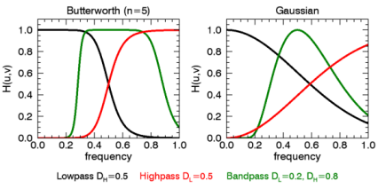
Here, we plot the frequency response of the Butterworth (n=5) and Gaussian filters. For the lowpass filter we use a high-frequency cut-off of 0.5, for highpass we use a cut-off of 0.5, and for the bandpass we use DL=0.2 and DH=0.8.
m = [0.2,0.27,0.05,0.1]
p = PLOT('1/(1 + (X/0.5)^10)', '3', DIM=[600,300], FONT_SIZE=10, $
XRANGE=[0,1], YRANGE=[0,1.1], LAYOUT=[2,1,1], MARGIN=m, $
XTITLE='frequency', YTITLE='H(u,v)', TITLE='Butterworth (n=5)')
p = PLOT('1-1/(1 + (X*0.6/(X^2-0.5^2))^10)', '3g', /OVERPLOT)
p = PLOT('1/(1 + (0.5/X)^10)', '3r', /OVERPLOT)
p = PLOT('exp(-X^2/(2*0.5^2))', '3', DIM=[600,300], FONT_SIZE=10, $
XRANGE=[0,1], YRANGE=[0,1.1], LAYOUT=[2,1,2], MARGIN=m, $
XTITLE='frequency', YTITLE='H(u,v)', TITLE='Gaussian', /CURRENT)
p = PLOT('exp(-((X^2-0.5^2)/(X*0.6))^2)', '3g', /OVERPLOT)
p = PLOT('1-exp(-X^2/(2*0.5^2))', '3r', /OVERPLOT)
t = TEXT(0.15,0.05,'Lowpass $D_H=0.5$',/NORM, FONT_SIZE=9)
t = TEXT(0.37,0.05,'Highpass $D_L=0.5$',COLOR='red',/NORM, FONT_SIZE=9)
t = TEXT(0.6,0.05,'Bandpass $D_L=0.2, D_H=0.8$',COLOR='green',/NORM, FONT_SIZE=9)
p.Save, 'bandpass_filter.png', resolution=120
In the following example, we add some sinusoidal noise to an image and filter it with BANDPASS_FILTER, using the BUTTERWORTH keyword.
; Read in the file
File = FILEPATH('moon_landing.png', SUBDIR=['examples','data'])
ImageOriginal = READ PNG(file)
; Generate some sinusoidal noise
XCoords = LINDGEN(300,300) MOD 300
YCoords = TRANSPOSE(xCoords)
Noise = -SIN(xCoords*2)-SIN(yCoords*2)
ImageNoise = imageOriginal + 50*noise
; Filter using a lowpass filter
ImageFiltered = BANDPASS FILTER(imageNoise, 0, 0.4, $
BUTTERWORTH=20)
; Display the original, noise-added, and filtered images
i=IMAGE(imageOriginal, LAYOUT=[3,1,1], TITLE='Original Image', $
DIMENSIONS=[700,300])
i=IMAGE(imageNoise, LAYOUT=[3,1,2], /CURRENT, TITLE='Added Noise')
i=IMAGE(imageFiltered, LAYOUT=[3,1,3], /CURRENT, $
TITLE='Butterworth Filtered')
i.Save, 'bandpass_filter_butterworth_ex.gif', resolution=120
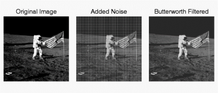
Key takeaway
The BANDPASS_FILTER function applies a lowpass, bandpass, or highpass filter to a one-channel image.
A bandpass filter is useful when the general location of the noise in the frequency domain is known. The bandpass filter allows frequencies within the chosen range through and attenuates frequencies outside of the given range.
Notch filters:
- Are used to remove repetitive "Spectral" noise from an image
- Are like a narrow highpass filter, but they "notch" out frequencies other than the dc component
- Attenuate a selected frequency (and some of its neighbors) and leave other frequencies of the Fourier to transform relatively unchanged
Repetitive noise in an image is sometimes seen as a bright peak somewhere other than the origin. You can suppress such noise effectively by carefully erasing the peaks. One way to do this is to use a notch filter to simply remove that frequency from the picture. This technique is very common in sound signal processing where it is used to remove mechanical or electronic hum, such as the 60Hz hum from AC power. Although it is possible to create notch filters for common noise patterns, in general notch filtering is an ad hoc procedure requiring a human expert to determine what frequencies need to be removed to clean up the signal.
The following is an example of removing synthetic spectral "noise" from an image.
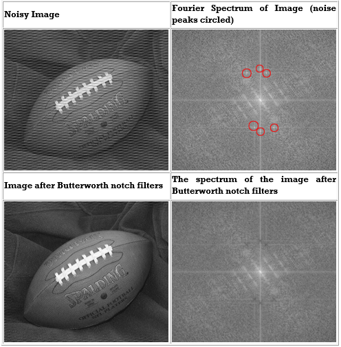
The above images were created using four M-files(paddedsize.m, lpfilter.m, dftuv.m, and notch.m), noiseball.png, and the following MATLAB calls
FootBall=imread('noiseball.png');
Imshow(footBall)
%Determine good padding for Fourier transform
PQ = paddedsize(size(footBall));
%Create Notch filters corresponding to extra peaks in the Fourier transform
H1 = notch('btw', PQ(1), PQ(2), 10, 50, 100);
H2 = notch('btw', PQ(1), PQ(2), 10, 1, 400);
H3 = notch('btw', PQ(1), PQ(2), 10, 620, 100);
H4 = notch('btw', PQ(1), PQ(2), 10, 22, 414);
H5 = notch('btw', PQ(1), PQ(2), 10, 592, 414);
H6 = notch('btw', PQ(1), PQ(2), 10, 1, 114);
% Calculate the discrete Fourier transform of the image
F=fft2(double(footBall),PQ(1),PQ(2));
% Apply the notch filters to the Fourier spectrum of the image
FS_football = F.*H1.*H2.*H3.*H4.*H5.*H6;
% convert the result to the spatial domain.
F_football=real(ifft2(FS_football));
% Crop the image to undo padding
F_football=F_football(1:size(footBall,1), 1:size(footBall,2));
%Display the blurred image
Figure, imshow(F_football,[])
% Display the Fourier Spectrum
% Move the origin of the transform to the center of the frequency rectangle.
Fc=fftshift(F);
Fcf=fftshift(FS_football);
% use abs to compute the magnitude and use log to brighten display
S1=log(1+abs(Fc));
S2=log(1+abs(Fcf));
Figure, imshow(S1,[])
Figure, imshow(S2,[])
Key takeaway
Notch filters:
- Are used to remove repetitive "Spectral" noise from an image
- Are like a narrow highpass filter, but they "notch" out frequencies other than the dc component
- Attenuate a selected frequency (and some of its neighbors) and leave other frequencies of the Fourier to transform relatively unchanged
When several interference components are present or if the interference has broad skirts a simply notch filter may remove too much image information.
One solution is to use an optimum filter that minimizes local variances of the restoredestimate.
Such “smoothness” constraints are often found in optimum filter design
1. Manually place a notch pass filter HNP at each noise spike in the frequency domain. The Fourier transform of the interference noise pattern is

2. Determine the noise pattern in the spatial domain

3. Conventional thinking would be to simply eliminate noise by subtracting the periodic noise from the noisy image

4. To construct an optimal filter consider

Where w (x, y) is a weighting function.
5. We use the weighting function w (x, y) to minimizethe variance 2(x, y) with respect to w (x, y)
We only need to compute this for one point in each non-overlapping neighborhood.

g (x, y) n (x, y) Mean product of noisy images and noise
n (x, y) Mean noise output from the notch filter
n2(x, y) Mean squared noise output from the notch filter
Key takeaway
When several interference components are present or if the interference has broad skirts a simply notch filter may remove too much image information.
One solution is to use an optimum filter that minimizes local variances of the restored estimate.
Such “smoothness” constraints are often found in optimum filter design
•If a degraded image is given by degradation + noise

•Estimate the image by dividing by the degradation function H (u, v)

We can never recover F (u, v) exactly:
1.N(u, v) is not known since (x, y) is a r.v. — estimated
2.If H (u, v) ->0 then the noise term will dominate. Helped byrestricting the analysis to (u, v) near the origin.
Modeling of Degradation
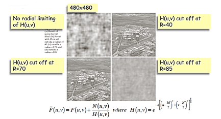
Minimize e2 = E{ ( f- F᷈)2}
Assuming
1. F and n are uncorrelated
2. f and/ or n is zero mean
3. Gray levels in f are a linear function of the gray levels in f
The best estimate F᷈ (u, v) is then given by
F᷈ (u, v) = [ H*(u, v) Sf (u, v) / Sf (u, v) |H(u, v)|2 + Sn (u, v)] G(u, v) = [ H*(u, v) / |H(u, v)|2 + Sn (u, v)/ Sf (u, v) ] G(u, v)
F᷈ (u, v) = [1/H(u, v) × |H(u, v)|2 / |H(u, v)|2 + Sn(u, v) / Sf (u, v) ] G(u, v)
H(u, v) = degradation function
H*(u, v) = complex conjugate of H
|H(u, v)| = H*(u, v) H(u, v)
Sn(u, v) = |N(u, v)|2 = power spectrum of noise (estimated)
Sf (u, v) = |F(u, v)|2 = power spectrum of original image (not known)
Modeling of Degradation
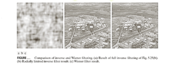
Inverse filtering

Radially limit at D0 = 75
Wiener filtering

In practice we don’t know the power spectrum Sf(u, v) = |F(u, v)|2 of the original image so we replace the  / Sf term with a constant K which we vary
Simple thresholding
Consider this image, with a series of crudely cut shapes set against a white background. The black outline around the image is not part of the image.
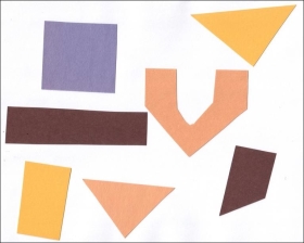
Now suppose we want to select only the shapes from the image. In other words, we want to leave the pixels belonging to the shapes “on,” while turning the rest of the pixels “off,” by setting their color channel values to zeros. The skimage library has several different methods of thresholding. We will start with the simplest version, which involves an important step of human input. Specifically, in this simple, fixed-level thresholding, we have to provide a threshold value, t.
The process works like this. First, we will load the original image, convert it to grayscale, and blur it with one of the methods from the Blurring episode. Then, we will use the > operator to apply the threshold t, a number in the closed range [0.0, 1.0]. Pixels with color values on one side of t will be turned “on,” while pixels with color values on the other side will be turned “off.” To use this function, we have to determine a good value for t. How might we do that? Well, one way is to look at a grayscale histogram of the image. Here is the histogram produced by the GrayscaleHistogram.py program from the Creating Histograms episode, if we run it on the image of the colored shape shown above.
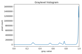
Since the image has a white background, most of the pixels in the image are white. This corresponds nicely to what we see in the histogram: there is a spike near the value of 1.0. If we want to select the shapes and not the background, we want to turn off the white background pixels, while leaving the pixels for the shapes turned on. So, we should choose a value of t somewhere before the large peak and turn pixels above that value “off”.
Here are the first few lines of a Python program to apply simple thresholding to the image, to accomplish this task.
"""
* Python script to demonstrate simple thresholding.
*
* usage: python Threshold.py <filename><sigma><threshold>
"""
Import sys
Import numpy as np
Import skimage.color
Import skimage.filters
Import skimage.io
Import skimage.viewer
# get filename, sigma, and threshold value from command line
Filename = sys.argv[1]
Sigma = float(sys.argv[2])
t = float(sys.argv[3])
# read and display the original image
Image = skimage.io.imread(fname=filename)
Viewer = skimage.viewer.ImageViewer(image)
Viewer.show()
This program takes three command-line arguments: the filename of the image to manipulate, the sigma of the Gaussian used during the blurring step (which, if you recall from the Blurring episode, must be a float), and finally, the threshold value t, which should be a float in the closed range [0.0, 1.0]. The program takes the command-line values and stores them in variables named filename, sigma, and t, respectively.
Next, the program reads the original image based on the filename value and displays it.
Now is where the main work of the program takes place.
# blur and grayscale before thresholding
Blur = skimage.color.rgb2gray(image)
Blur = skimage.filters.gaussian(blur, sigma=k)
First, we convert the image to grayscale and then blur it, using the skimage.filter.gaussian() function we learned about in the Blurring episode. We convert the input image to grayscale for easier thresholding.
The fixed-level thresholding is performed using numpy comparison operators.
# perform inverse binary thresholding
Mask = blur <t_rescaled
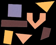
Here, we want to turn “on” all pixels that have values smaller than the threshold, so we use the less operator < to compare the blurred image blur to the threshold t. The operator returns a binary image, that we capture in the variable mask. It has only one channel, and each of its values is either 0 or 1. Here is a visualization of the binary image created by the thresholding operation. The program used parameters of sigma = 2 and t = 0.8 to produce this image. You can see that the areas where the shapes were in the original area are now white, while the rest of the mask image is black.

We can now apply the mask to the original-colored image as we have learned in the Drawing and Bitwise Operations episode.
# use the mask to select the "interesting" part of the image
Sel = np.zeros_like(image)
Sel[mask] = image[mask]
# display the result
Viewer = skimage.viewer.ImageViewer(sel)
Viewer.view()
What we are left with is only the colored shapes from the original, as shown in this image:
More practice with simple thresholding (15 min)
Now, it is your turn to practice. Suppose we want to use simple thresholding to select only the colored shapes from this image:
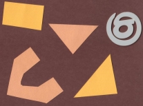
First, use the GrayscaleHistogram.py program in the Desktop/workshops/image-processing/05-creating-histograms directory to examine the grayscale histogram of the more-junk.jpg image, which you will find in the
Desktop/workshops/image-processing/07-thresholding directory.
Via the histogram, what do you think would be a good value for the threshold value, t?
Solution
Now, modify the ThresholdPractice.py program in the
Desktop/workshops/image-processing/07-thresholding directory to turn the pixels above the t value on and turn the pixels below the t value off. To do this, change the comparison operator less <to greater >. Then execute the program on the more-junk.jpg image, using a reasonable value for k and the t value you obtained from the histogram. If everything works as it should, your output should show only the colored shapes on a pure black background.
Solution
Adaptive thresholding
There are also skimage methods to perform adaptive thresholding. The chief advantage of adaptive thresholding is that the value of the threshold, t, is determined automatically for us. One such method, Otsu’s method, is particularly useful for situations where the grayscale histogram of an image has two peaks. Consider this maize root system image, which we have seen before in the Skimage Images episode.
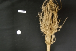
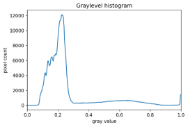
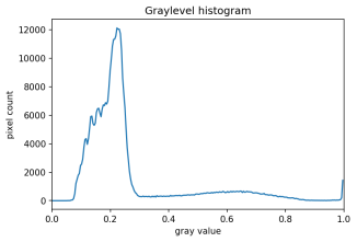
Now, look at the grayscale histogram of this image, as produced by our GrayscaleHistogram.py program from the Creating Histograms episode.
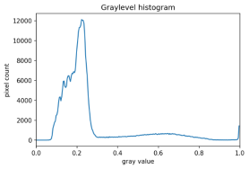
The histogram has a significant peak around 0.2, and a second, albeit smaller peak very near 1.0. Thus, this image is a good candidate for thresholding with Otsu’s method. The mathematical details of how these works are complicated (see the skimage documentation if you are interested), but the outcome is that Otsu’s method finds a threshold value between the two peaks of a grayscale histogram.
The skimage.filters.threshold_otsu() function can be used to determine the adaptive threshold via Otsu’s method. Then numpy comparison operators can be used to apply it as before.
Here is a Python program illustrating how to perform thresholding with Otsu’s method using the skimage.filters.threshold_otsu function. We start by reading and displaying the target image.
"""
* Python script to demonstrate adaptive thresholding using Otsu's method.
*
* usage: python AdaptiveThreshold.py <filename><sigma>
"""
Import sys
Import numpy as np
Import skimage.color
Import skimage.filters
Import skimage.io
Import skimage.viewer
# get filename and sigma value from command line
Filename = sys.argv[1]
Sigma = float(sys.argv[2])
# read and display the original image
Image = skimage.io.imread(fname=filename)
Viewer = skimage.viewer.ImageViewer(image)
Viewer.show()
The program begins with the now-familiar imports and command-line parameters. Here we only have to get the filename and the sigma of the Gaussian kernel from the command line, since Otsu’s method will automatically determine the thresholding value t. Then, the original image is read and displayed.
Next, a blurred grayscale image is created.
# blur and grayscale before thresholding
Blur = skimage.color.rgb2gray(image)
Blur = skimage.filters.gaussian(image, sigma=sigma)
We determine the threshold via the skimage.filters.threshold_otsu() function:
# perform adaptive thresholding
t = skimage.filters.threshold_otsu(blur)
Mask = blur > t
The function skimage.filters.threshold_otsu() uses Otsu’s method to automatically determine the threshold value based on its inputs grayscale histogram and returns it. Then, we use the comparison operator > for binary the holding. As we have seen before, pixels above the threshold value will be turned on, those below the threshold will be turned off.
For this root image, and a Gaussian blur with a sigma of 1.0, the computed threshold value is 0.42, and the resulting mask is:
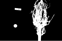
Next, we display the mask and use it to select the foreground
Viewer = skimage.viewer.ImageViewer(mask)
Viewer.show()
# use the mask to select the "interesting" part of the image
Sel = np.zeros_like(image)
Sel[mask] = image[mask]
# display the result
Viewer = skimage.viewer.ImageViewer(sel)
Viewer.show()
Here is the result:
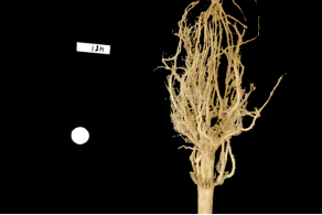
Application: measuring root mass
Let us now turn to an application where we can apply thresholding and other techniques we have learned to this point. Consider these four maize root system images.
Now suppose we are interested in the amount of plant material in each image, and in particular how that amount changes from image to image. Perhaps the images represent the growth of the plant over time, or perhaps the images show four different maize varieties at the same phase of their growth. In any case, the question we would like to answer is, “how much root mass is in each image?” We will construct a Python program to measure this value for a single image, and then create a Bash script to execute the program on each trial image in turn.
Our strategy will be this:
- Read the image, converting it to grayscale as it is read. For this application, we do not need the color image.
- Blur the image.
- Use Otsu’s method of thresholding to create a binary image, where the pixels that were part of the maize plant are white, and everything else is black.
- Save the binary image so it can be examined later.
- Count the white pixels in the binary image, and divide by the number of pixels in the image. This ratio will be a measure of the root mass of the plant in the image.
- Output the name of the image processed and the root mass ratio.
Here is a Python program to implement this root-mass-measuring strategy. Almost all of the code should be familiar, and in fact, it may seem simpler than the code we have worked on thus far because we are not displaying any of the images with this program. Our program here is intended to run and produce its numeric result – a measure of the root mass in the image – without human intervention.
"""
* Python program to determine root mass, as a ratio of pixels in the
* root system to the number of pixels in the entire image.
*
* usage: python RootMass.py <filename><sigma>
"""
Import sys
Import numpy as np
Import skimage.io
Import skimage.filters
# get filename and sigma value from command line
Filename = sys.argv[1]
Sigma = float(sys.argv[2])
# read the original image, converting to grayscale
Img = skimage.io.imread(fname=filename, as_gray=True)
The program begins with the usual imports and reading of command-line parameters. Then, we read the original image, based on the filename parameter, in grayscale.
Next, the grayscale image is blurred with a Gaussian that is defined by the sigma parameter.
# blur before thresholding
Blur = skimage.filters.gaussian(img, sigma=sigma)
Following that, we create a binary image with Otsu’s method for thresholding, just as we did in the previous section. Since the program is intended to produce numeric output, without a person shepherding it, it does not display any of the images.
# perform adaptive thresholding to produce a binary image
t = skimage.filters.threshold_otsu(blur)
Binary = blur > t
We do, however, want to save the binary images, in case we wish to examine them at a later time. That is what this block of code does:
# save binary image; first find beginning of file extension
Dot = filename.index(".")
Binary_file_name = filename[:dot] + "-binary" + filename[dot:]
Skimage.io.imsave(fname=binary_file_name, arr=skimage.img_as_ubyte(binary))
This code does a little bit of string manipulation to determine the filename to use when the binary image is saved. For example, if the input filename being processed is trial-020.jpg, we want to save the corresponding binary image as trial-020-binary.jpg. To do that, we first determine the index of the dot between the filename and extension – and note that we assume that there is only one dot in the filename! Once we have the location of the dot, we can use slicing to pull apart the filename string, inserting “-binary” in between the end of the original name and the extension. Then, the binary image is saved via a call to the skimage.io.imsave() function. In order to convert from the binary range of 0 and 1 of the mask to a gray level image that can be saved as png, we use the skimage.img_as_ubyte utility function.
Finally, we can examine the code that is the reason this program exists! This block of code determines the root mass ratio in the image:
# determine root mass ratio
RootPixels = np.nonzero(binary)
w = binary.shape[1]
h = binary.shape[0]
Density = rootPixels / (w * h)
# output in format suitable for .csv
Print(filename, density, sep=",")
Recall that we are working with a binary image at this point; every pixel in the image is either zero (black) or 1 (white). We want to count the number of white pixels, which is easily accomplished with a call to the np.count_nonzero function. Then we determine the width and height of the image, via the first and second elements of the image’s shape. Then the density ratio is calculated by dividing the number of white pixels by the total number of pixels in the image. Then, the program prints out the name of the file processed and the corresponding root density.
If we run the program on the trial-016.jpg image, with a sigma value of 1.5, we would execute the program this way:
Python RootMass.py trial-016.jpg 1.5
And the output we would see would be this:
Trial-016.jpg,0.0482436835106383
We have four images to process in this example, and in a real-world scientific situation, there might be dozens, hundreds, or even thousands of images to process. To save us the tedium of running the Python program on each image, we can construct a Bash shell script to run the program multiple times for us. Here is a sample script, which assumes that the images all start with the trial- prefix, and end with the .jpg file extension. The script also assumes that the images, the RootMass.py program, and the script itself are all in the same directory.
#!/bin/bash
# Run the root density mass on all of the root system trail images.
# first, remove existing binary output images
Rm *-binary.jpg
# then, execute the program on all the trail images
For f in trial-*.jpg
Do
Python RootMass.py $f 1.5
Done
The script begins by deleting any prior versions of the binary images. After that, the script uses a for loop to iterate through all of the input images, and execute the RootMass.py on each image with a sigma of 1.5. When we execute the script from the command line, we will see output like this:
Trial-016.jpg,0.0482436835106383
Trial-020.jpg,0.06346941489361702
Trial-216.jpg,0.14073969414893617
Trial-293.jpg,0.13607895611702128
It would probably be wise to save the output of our multiple runs to a file that we can analyze later on. We can do that very easily by redirecting the output stream that would normally appear on the screen to a file. Assuming the shell script is named rootmass.sh, this would do the trick:
Bash rootmass.sh > rootmass.csv
Ignoring more of the images – brainstorming (10 min)
Let us take a closer look at the binary images produced by the proceeding program.
Our root mass ratios include white pixels that are not part of the plant in the image, do they not? The numbered labels and the white circles in each image are preserved during the thresholding, and therefore their pixels are included in our calculations. Those extra pixels might have a slight impact on our root mass ratios, especially the labels since the labels are not the same size in each image. How might we remove the labels and circles before calculating the ratio, so that our results are more accurate? Brainstorm and think about some options, given what we have learned so far.
Solution
Ignoring more of the images – implementation (30 min)
Navigate to the Desktop/workshops/image-processing/07-thresholding directory, and edit the RootMassImproved.py program. This is a copy of the RootMass.py program developed above. Modify the program to apply simple inverse binary thresholding to remove the white circle and label from the image before applying Otsu’s method. Comments in the program show you where you should make your changes.
Solution
Thresholding a bacteria colony image (10 min)
In the Desktop/workshops/image-processing/07-thresholding directory, you will find an image named colonies01.tif; this is one of the images you will be working within the morphometric challenge at the end of the workshop. First, create a grayscale histogram of the image, and determine a threshold value for the image. Then, write a Python program to threshold a grayscale version of the image, leaving the pixels in the bacteria colonies “on,” while turning the rest of the pixels in the image “off.”
Key Points
- Thresholding produces a binary image, where all pixels with intensities above (or below) a threshold value are turned on, while all other pixels are turned off.
- The binary images produced by thresholding are held in two-dimensional NumPy arrays since they have only one color value channel. They are boolean, hence they contain the values 0 (off) and 1 (on).
- Thresholding can be used to create masks that select only the interesting parts of an image, or as the first step before Edge Detection or finding Contours.
Key takeaway
Now suppose we want to select only the shapes from the image. In other words, we want to leave the pixels belonging to the shapes “on,” while turning the rest of the pixels “off,” by setting their color channel values to zeros. The skimage library has several different methods of thresholding. We will start with the simplest version, which involves an important step of human input. Specifically, in this simple, fixed-level thresholding, we have to provide a threshold value, t.
References:
1. Rafael C. Gonzalez, Richard E. Woods, Digital Image Processing Pearson, Third Edition, 2010
2. Anil K. Jain, Fundamentals of Digital Image Processing Pearson, 2002.
3. Kenneth R. Castleman, Digital Image Processing Pearson, 2006.
4. Rafael C. Gonzalez, Richard E. Woods, Steven Eddins, Digital Image Processing using MATLAB Pearson Education, Inc., 2011.
5. D, E. Dudgeon, and RM. Mersereau, Multidimensional Digital Signal Processing Prentice Hall Professional Technical Reference, 1990.
6. William K. Pratt, Digital Image Processing John Wiley, New York, 2002
7. Milan Sonka et al Image processing, analysis and machine vision Brookes/Cole, Vikas Publishing House, 2nd edition, 1999