Unit - 2

Numerical Method

2.1 Finite difference

The calculus of finite differences deals with the changes that take place in the value of the function (dependent variable) due to finite changes in the independent variable.

Suppose, we are given a set of values (xi, yi); i = 1, 2, 3, ......, n of any function y = f(x).

A value of independent variable x is called argument and the corresponding value of dependent variable y is called entry.

Finite Difference:

Let be a function of x. The table given below gives corresponding values of y for different values of x.

X				….
y= f(x)				….

Forward Difference: 

Then  are called differences of y, denoted by 

The symbol is called the forward difference operator.  Consider the forward difference table below:

Where

And third forward difference so on.

Backward Difference:

The difference are called first backward difference and  is denoted by  Consider the backward  difference  table  below:

Where

And third backward differences so on.

Key takeaways-

1. Interpolation is a technique of  estimating the value of  a  function for any  intermediate value of the  independent  variable while  the process  of  computing the  value of the function outside the given range is called   extrapolation.
2. If the given function is a polynomial it is polynomial interpolation and given function is known as interpolating polynomial.

a)     Forward Difference:  The  are called differences of y, denoted by 

The symbol  is  called the forward  difference operator

3.     Backward Difference:

The difference are called first  backward difference and  is denoted by 

2.2 Symbolic relations

Shift operator E

It is the operation of increasing the argument x by h so that

Ef(x) = f(x + h)

E2f(x) = f(x + 2h) and so on.

The inverse operator is defined by

Also

Averaging operator

It is defined by

Relation between operators:

Proof:

We know that,

Or

2.    

Proof:

3.    

Proof:

4.    

Proof:

5.    

Proof:

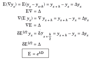
6.    

Proof:

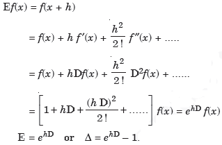
Note-

Table

Example: Show that

Sol:

Example: Show that

Sol:

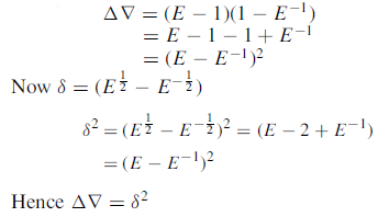
Example: Prove that

Sol:

Key takeaways:

2.3 Interpolation, Newton - Gregory forward and backward formula

Definition:

Interpolation is a technique of estimating the value of a function for any intermediate value of the independent variable while the process of computing the value of the function outside the given range is called   extrapolation.

Let be a function of x.

The table given below gives corresponding values of y for different values of x.

X    …. 

y= f(x)    …. 

The process of finding the values of y corresponding to any value of x which lies between   is called interpolation.

If the given function is a polynomial, it is polynomial interpolation and given function is known as interpolating polynomial.

Note- The process of computing the value of the function outside the given range is called extrapolation.

Thus, interpolation is the “art of reading between the lines of a table.”

Conditions for Interpolation

1)     The function must be   a polynomial of independent variable.

2)     The function   should be either increasing or decreasing function.

3)     The value of   the function should be increase or decrease uniformly.

Finite Difference

Let be a function of x. The table given below gives corresponding values of y for different values of x.

X    …. 

y= f(x)    …. 

There are three types of differences are useful-

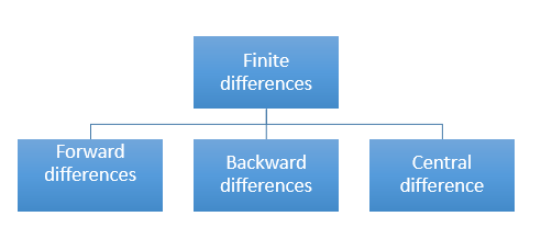
b)    Forward Difference:
The  are called differences of y, denoted by 

The symbol   is called the forward difference operator.  Consider the forward difference table below:

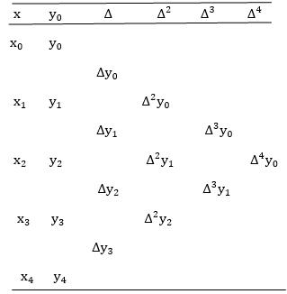
Where

And third forward difference so on.

c)     Backward Difference:

The difference are called first backward difference and is denoted by  Consider the backward difference table below:

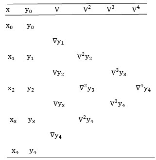
Where

And third backward differences so on.

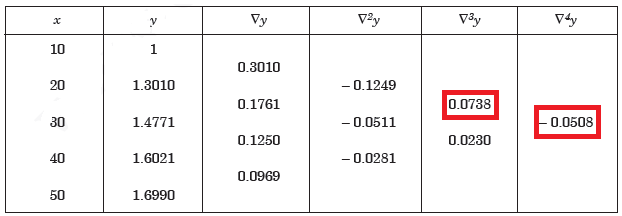
Example: Construct a backward difference table for y = log x, given-

Sol. The backward difference table will be-

Newton Forward Difference formula:

This method is useful for interpolation near the beginning of a set of tabular values.

Where

Example1: Using Newton’s forward difference formula, find the sum

Putting

It   follows that

Since is a fourth-degree polynomial in n.

Further,

By Newton Forward Difference Method

Example2: Given  find   , by using Newton forward interpolation method.

Let , then

	0.7071	0.7660	-	0.8192	0.8660

The table of forward finite difference is given below:

45           50           55            60	0.7071            0.7660           0.8192            0.8660	0.0589          0.0532          0.0468	-0.0057        -0.0064	-0.0007

By Newton forward difference method

Here initial value = 45, difference of interval h = 5 and the value to be calculated at x=52.

By Formula

Example3: Find the missing term in the following:

	0	1	2	3	4
	1	3	9	?	81

Let

First, we construct the forward difference table:

0       1        2        3        4	1       3       9         81	2         6	4

Now,

Newton Backward Difference Method:

This method is useful for interpolation near the ending of a set of tabular values.

Where 

Example1:  Find from the following table:

	0.20	0.22	0.24	0.26	0.28	0.30
	1.6596	1.6698	1.6804	1.6912	1.7024	1.7139

Consider the backward difference method

0.20         0.22         0.24         0.26         0.28         0.30	1.6596      1.6698      1.6804      1.6912     1.7024       1.7139	0.0102       0.0106      0.0108      0.0112     0.0115	0.0004    0.0002    0.0004    0.0003	-0.0002    0.0002   -0.0001	0.0004   -0.0003	-0.0007

Here

By Newton backward difference formula

Example2: The following table give the amount of a chemical dissolved in water:

Temp.
Solubility	19.97	21.51	22.47	23.52	24.65	25.89

Compute the amount dissolve at

Consider the following backward difference table:

Temp.  x	Solubility y
10     15     20     25     30     35	19.97      21.51     22.47     23.52      24.65      25.89	1.54     0.96    1.05     1.13     1.24	-0.58      0.09      0.08      0.11	0.67     -0.01      0.03	-0.68     0.04	0.72

Here

By Newton Backward difference formula

Example3: The following are the marks obtained by 492 candidates in a certain examination

Find out the number of candidates:

a)     Who secured more than 48 but not more than 50 marks?

b)    Who secured less than 48 but not less than 45 marks?

Consider the forward difference table given below:

Marks up to x	No. Of candidates y
40       45       50       55       60       65	210   210+43=253   253+54=307   307+74=381   381+32=413   413+79= 492	43       54       74       32        79	11     20     -42      47	9     -62      89	-71        151	222

Here 

By Newton Forward Difference formula

f

a)     No. Of candidate secured more than 48 but not more than 50 marks

b)    No. Of candidate secured less than 48 but not less than 45 marks

Key takeaways-

1. Interpolation is a technique of estimating the value of a function for any intermediate value of the independent variable while the process of computing the value of the function outside the given range is called   extrapolation.
2. If the given function is a polynomial, it is polynomial interpolation and given function is known as interpolating polynomial.
3. Forward Difference:  The  are called differences of y, denoted by 

The symbol  is called the forward difference operator

4.     Backward Difference:

The difference are called first backward difference and is denoted by 

5.     Newton Forward Difference formula:

Where

6.     Newton Backward Difference Method:

Where 

2.4 Extrapolation

Interpolation is the technique of estimating the value of a function for any intermediate value of the independent variable while the process of computing the value of

The function outside the given range is called extrapolation.

In other words- “Extrapolation is defined as an estimation of a value based on extending the known series or factors beyond the area that is certainly known. In other words, extrapolation is a method in which the data values are considered as points such as x1, x2, ….., xn.”

2.5 Lagrange's formula

Lagrange’s interpolation of polynomial:

Let , be defined function we get

X				…..
f(x)				……

Where the interval is not necessarily equal. We assume f(x) is a polynomial od degree n.  Then Lagrange’s interpolation formula is given by

Example1: Deduce Lagrange’s formula for interpolation.  The observed values of a function are respectively 168,120,72 and 63 at the four position3,7,9 and 10 of the independent variables. What is the best estimate you can for the value of the function at the position6 of the independent variable?

We construct the table for the given data:

We need to calculate for x = 6, we need f (6) =?

Here

We get

By Lagrange’s interpolation formula, we have

Hence the estimated value for x=6 is 147.

Example2:By means of Lagrange’s formula, prove that

We construct the table:

X	0	1	2	3	4	5	6
Y=f(x)

Here x = 3, f(x)=?

By Lagrange’s formula for   interpolation

Hence proved.

Example3: find the polynomial of fifth degree from the following data

Here

We get 

By Lagrange’s interpolation formula

Key takeaways

Then Lagrange’s interpolation formula is-

2.6 Inverse Interpolation by Lagrange's formula

Overview:

In the inverse interpolation, for a given value of y, the corresponding value of x is to be determined.

e.g.- To find value of the root x for which the function y = f (x) becomes zero is an inverse interpolation problem. Inverse interpolation problem is similar to direct interpolation since the roles of x and y are interchanged.

Inverse Interpolation (Lagrange’s Method)

Given a set of values of x and y, the process of finding the value of x  for a certain value of y is called inverse interpolation.

Lagrange’s Inverse interpolation:

Let , be  defined  function we get

x				…..
f(Y)				……

Where the interval is not necessarily equal. We assume f(x) is a polynomial of degree n.  Then Lagrange’s inverse interpolation formula is given by

Example1: Use the inverse interpolation to find value of x at for the following data:

Here , we have the  data

The Lagrange’s inverse interpolation formula is given by

.

Example2: Use the inverse   Lagrange’s method to find the root of the equation , give data

Here , we have the  data

Also.

The Lagrange’s inverse interpolation formula is given by

Thus the approximate   root of the given equation is .

Example3: Find the value of x at for the following data:

Here , we have the  data

Also.

The Lagrange’s inverse interpolation formula is given by

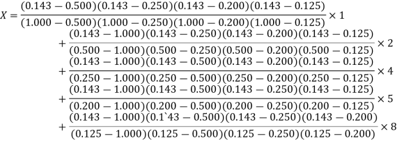
Thus the value

Key takeaways:

Then Lagrange’s inverse interpolation formula is given by

2.7 Numerical Differentiation and Numerical Integration

Numerical differentiation:

Overview:

In the case of numerical data, the functional form of f(x) is not known in general. First we have to find an appropriate form of f(x) and then obtain its derivatives. So “Numerical differentiation” is used to find the successive derivatives of a function at a given argument, using the given table of entries corresponding to a set of arguments, equally or unequally spaced. Using the theory of interpolation, a suitable interpolating polynomial can be chosen to represent the function to a good degree of approximation in the given interval of the argument.

For the proper choice of interpolation formula, the criterion is same as in case of interpolation problems. In case of equidistant values of x, if the derivative is to be found at a point near the beginning or the end of the given set of values, we should use Newton’s forward or backward difference formula accordingly. Also if the derivative is to be found at a point near the middle of the given set of values, then we should use any one of the central difference formulae. However, if the values of the function are not known at equidistant values of x, we shall use Newton’s divided difference or Lagrange’s formula.

Newton’s forward Difference formula:

This method is useful for interpolation near the beginning of a set of tabular values.

Where
 

Differentiating both side with respect to p, we get

h

This formula is applicable to compute the value of for non tabular values of x.

For tabular values of x , we can get formula by putting 

Therefore

In similar manner we can get the formula for higher order by differentiating the previous order formulas

Again differentiating with respect to p, we get

Hence

Also

And so on.

Example1: Given that

Find at .

Here the first derivative is to be calculated at the beginning of the table, therefore  forward difference  formula will be used

Forward difference table is given below:

X	Y
1.0   1.1   1.2   1.3	0.841   0.891   0.932   0.962	0.050   0.041   0.031	-0.009   -0.010	-0.001

By Newton’s forward differentiation formula for differentiation

Here 

Example2: Find the first and second  derivatives of the function given below at the  point :

Here the point of the calculation is  at the beginning of the  table,

Forward difference table is given  by:

X	Y
1   2   3   4   5	0   1   5   6   8	1   4   1   2	3   -3   1	-6   4	-10

By Newton’s forward differentiation formula for differentiation

Here  , 0.

Again 

At

Example3: From the following  table of values of x and y find   for 

Here the  value of the derivative is to be  calculated at  the beginning of the table.

Forward difference table is given by

X	Y
1.00   1.05   1.10   1.15   1.20   1.25   1.30	1.0000   1.02470   1.04881   1.07238   1.09544   1.11803   1.14017	0.02470   0.02411   0.02357   0.02306   0.02259   0.02214	-0.00059   -0.00054   -0.00051   -0.00047   -0.00045	0.00005   0.00003   0.00004   0.00002	-0.00002   0.00001   -0.00002	0.00003   -0.00003	-0.00006

From Newton’s forward difference formula for differentiation we get

Here

=0.48763

Newton Backward Difference Method:

This method is useful for interpolation near the ending of a set of tabular values.

Where 

Differentiating both side with respect to p, we get

This formula is applicable to compute the value of for non tabular values of x.

For tabular values of x , we can get formula by putting 

Therefore

In similar manner we can get the formula for higher order by differentiating the previous order formulas

Differentiating both side with respect to p, we get

Also

Example1: Given that

Find ?

Backward difference table:

X	Y
0.1   0.2   0.3   0.4	1.10517   1.22140   1.34986   1.49182	0.11623   0.12846   0.14196	0.01223   0.01350	0.00127

Newton’s Backward formula for differentiation

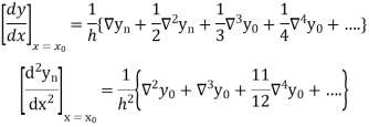
Here

Example2: Given that

Find the derivative of y at ?

The difference table is  given below:

X	Y
1.0   1.2   1.4   1.6   1.8   2.0	0   0.128   0.544   1.296   2.432   4.0	0.128   0.416   0.752   0.136   1.568	0.288   0.336   0.384   0.432	0.048   0.048   0.048	0   0

Since the point  is at the beginning of the table therefore

From Newton’s forward difference formula for differentiation we get

Here

Since the point is at the  end of the  table  therefore

Backward difference table is:

X	Y
1.0   1.2   1.4   1.6   1.8   2.0	0   0.128   0.544   1.296   2.432   4.000	0.128   0.416   0.752   0.136   1.568	0.288   0.336   0.384   0.432	0.048   0.048   0.048	0   0

Newton’s Backward formula for differentiation

Key takeaways:

1. Newton’s forward Difference formula:

Where

2.     Newton Backward Difference Method:

Where 

2.8 Newton Cotes Quadrature formula

Numerical Integration

Numerical integration is a process of evaluating or obtaining a definite integral from a set of numerical values of the integrand f(x).In case of function of single variable, the process is called quadrature.

Newton cotes formula-

Suppose where y takes the values

And let the integration interval (a,b) is divided into n equal sub-intervals, each of width h = b – a /n, so that,

...(1)

The above formula is known as Newton’s cotes formula.

This is also known as general quadrature formula.

Note- A number of important deductions viz. Trapezoidal rule, Simpson’s one-third and three-eighth rules, can be immediately deduced by putting n = 1, 2 and 3 respectively, in formula (1).

2.9 Trapezoidal rule

Numerical integration is a process of evaluating or obtaining a definite integral from a set of numerical values of the integrand f(x). In case of function of single variable, the process is called quadrature.

Trapezoidal Method:

Let the interval [a, b] be divided into n equal intervals such that <<…. <=b.

Here .

To find the value of .

Setting n=1, we get

Or I =

The above is known as Trapezoidal method.

Note: In this method second and higher difference are neglected and so f(x) is a polynomial of degree 1.

Geometrical Significance: The curve y=f(x), is replaced by n straight lines with the points ();() and ();…….;() and ().

The area bounded by the curve y=f(x), the ordinates ,and the x axis is approximately equivalent to the sum of the area of the n trapeziums obtained.

Example1: State the trapezoidal rule for finding an approximate area under the given curve. A curve is given by the points (x, y) given below:

(0, 23), (0.5, 19), (1.0, 14), (1.5, 11), (2.0, 12.5), (2.5, 16), (3.0, 19), (3.5, 20), (4.0, 20).

Estimate the area bounded by the curve, the x axis and the extreme ordinates.

We construct the data table:

Here length of interval h =0.5, initial value a = 0 and final value b = 4

By Trapezoidal method

Area of curve bounded on x axis =

Example2: Compute the value of  

Using the trapezoidal rule with h=0.5, 0.25 and 0.125.

Here

For h=0.5, we construct the data table:

By Trapezoidal rule

For h=0.25, we construct the data table:

By Trapezoidal rule

For h = 0.125, we construct the data table:

By Trapezoidal rule

[(1+0.5) +2(0.98461+0.94117+0.87671+0.8+0.71910+0.64+0.56637)]

Example3: Evaluate using trapezoidal rule with five ordinates

Here

We construct the data table:

X	0
Y	0	0.3693161	1.195328	1.7926992	1.477265	0

Key takeaways

1. Numerical integration is a process of evaluating or obtaining a definite integral from a set of numerical values of the integrand f(x).
2. 

2.10 Simpson's 1/3" rule and Simpson's 3/8" rule

Overview-

Generally fundamental theorem of calculus is used find the solution for definite integrals, but sometime integration becomes too hard to evaluate, numerical methods are used to find the approximated value of the integral.

Simpson’s rules are very useful in numerical integration to evaluate such integrals.

Here we will understand the concept of Simpson’s rule and evaluate integrals by using numerical technique of integration.

We find more accurate value of the integration by using Simpson’s rule than other methods

Simpson’s rule

We will study about Simpson’s one-third rule and Simpson’s three-eight rules.

But in order to get these two formulas, we should have to know about the general quadrature formula-

General quadrature formula-

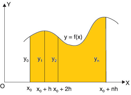
The general quadrature formula is gives as-

Simpson’s one-third and three-eighth formulas are derived by putting n = 2 and n = 3 respectively in general quadrature formula.

Simpson’s one-third and three-eighth formulas are derived by putting n = 2 and n = 3 respectively in general quadrature formula.

Simpson’s one-third rule-

Put n = 2 in general quadrature formula-

We get-

Note- the given interval of integration has to be divided into an even number of sub-intervals.

Simpson’s three-eighth rule-

Put n = 3 in general quadrature formula-

We get-

Note- the given interval of integration has to be divided into sub-intervals whose number n is a multiple of 3.

Example: Evaluate the following integral by using Simpson’s 1/3rd and 3/8th rule.

Solution-

First, we will divide the interval into six parts, where width (h) = 1, the value of f(x) is given in the table below-

x	0	1	2	3	4	5	6
f(x)	1	0.5	0.2	0.1	1/17 = 0.05884	1/26 = 0.0385	1/37 = 0.027

Now using Simpson’s 1/3rd rule-

We get-

And now

Now using Simpson’s 3/8th rule-

Example: Find the approximated value of the following integral by using Simpson’1/3rd rule.

Solution-

The table of the values-

x	1	1.25	1.5	1.75	2
f(x)	0.60653	0.53526	0.47237	0.41686	0.36788

Now using Simpson’s 1/3rd rule-

We get-

Example1: Estimate the value of the integral

By Simpson’s rule with 4 strips and 8 strips respectively.

For n=4, we have

E construct the data table:

By Simpson’s Rule

For n = 8, we have

By Simpson’s Rule

Example2: Evaluate Using Simpson’s 1/3 rule with .

For , we construct the data table:

X	0
	0	0.50874	0.707106	0.840896	0.930604	0.98281	1

By Simpson’s Rule

Example3: Using Simpson’s 1/3 rule with h = 1, evaluate

For h = 1, we construct the data table:

X	3	4	5	6	7
	9.88751	22.108709	40.23594	64.503340	95.34959

By Simpson’s Rule

= 177.3853

Example: Evaluate

By Simpson’s 3/8 rule.

Let us divide the range of the interval [4, 5.2] into six equal parts.

For h=0.2, we construct the data table:

By Simpson’s 3/8 rule 

= 1.8278475

Example2: Evaluate

Let us divide the range of the interval [0,6] into six equal parts.

For h=1, we construct the data table:

X	0	1	2	3	4	5	6
	1	0.5	0.2	0.1	0.0588	0.0385	0.027

By Simpson’s 3/8 rule

+3(0.0385) +0.027]

=1.3571

Error in Integration

Error in Trapezoidal method

The total error in trapezoidal method is given by

Let is the largest value of the n quantities on the right-hand side of the above equation then

Error in Simpson’s Rule

The error in the Simpson’s rule is given by

Where is the largest value of the fourth derivative of y(x).

Error in Simpson’s 3/8 Rule

The error in this rule is given by

Where is the largest value of the derivative of y(x).

Key takeaways

1. The general quadrature formula is gives as-

2.     Simpson’s one-third rule-

3.     Simpson’s three-eighth rule-

References:

1. R. J. Beerends H. G. Ter Morsche, J. C. Van Den Berg. L. M. Van De Vrie, Fourier and Laplace Transforms, Cambridge University Press.

2. Sastry S.S. Introductory Methods of Numerical Analysis, PHI.

3. B.S. Grewal: Higher Engineering Mathematics; Khanna Publishers, New Delhi.

4. B.V. Ramana: Higher Engineering Mathematics; Tata McGraw- Hill Publishing Company Limited, New Delhi.

5. Peter V.O’ Neil. Advanced Engineering Mathematics, Thomas (Cengage) Learning.