Unit - 2

Image Enhancement

2.1 Spatial Domain: Gray level transformations

All Image Processing Techniques focused on gray level transformation as it operates directly on pixels. The gray level image involves 256 levels of gray and in a histogram, the horizontal axis spans from 0 to 255, and the vertical axis depends on the number of pixels in the image.

The simplest formula for image enhancement technique is:

s = T * r  

Where T is transformation, r is the value of pixels, s is pixel value before and after processing.

Let,

1. r = f(x,y)  
2. s = g(x,y)  

'r' and 's' are used to denote gray levels of f and g at (x, y)

There are three types of transformation:

1. Linear
2. Logarithmic
3. Power - law

The overall graph is shown below:

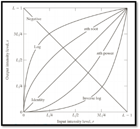
Fig 1 – Graph

Linear Transformation

The linear transformation includes identity transformation and negative transformation.

In identity transformation, each value of the image is directly mapped to each other values of the output image.

Negative transformation is the opposite of identity transformation. Here, each value of the input image is subtracted from L-1, and then it is mapped onto the output image

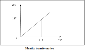
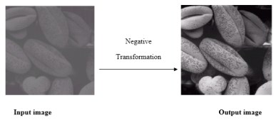
Fig 2 – Negative transformation

Logarithmic transformations

Logarithmic transformation is divided into two types:

1. Log transformation
2. Inverse log transformation

The formula for Logarithmic transformation

s = c log (r + 1)  

Here, s and r are the pixel values for input and output images. And c is constant. In the formula, we can see that 1 is added to each pixel value this is because if pixel intensity is zero in the image, then log (0) is infinity so, to have minimum value one is added.

When log transformation is done dark pixels are expanded as compared to higher pixel values. In the log transformation, higher pixels are compressed.

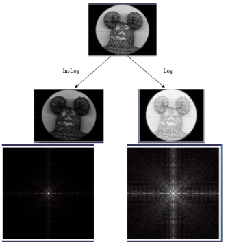
Fig 3 - In the above image (a) Fourier Spectrum and (b) result of applying Log Transformation.

Power - Law transformations

Power Law Transformation is of two types of transformation nth power transformation and nth root transformation.

Formula:

1. s = cr ^ γ  

Here, γ is gamma, by which this transformation is known as gamma transformation.

All display devices have their gamma correction. That is why images are displayed at different intensities.

These transformations are used for enhancing images.

For example:

Gamma of CRT is between 1.8 to 2.5

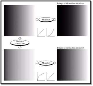
Fig 4 – Example

Image Enhancement

The main objective of Image Enhancement is to process the given image into a more suitable form for a specific application. It makes an image more noticeable by enhancing features such as edges, boundaries, or contrast. While enhancement, data does not increase, but the dynamic range is increased of the chosen features by which it can be detected easily.

In image enhancement, the difficulty arises to quantify the criterion for enhancement for which enhancement techniques are required to obtain satisfying results.

There are two types of Image enhancement methods:

1. Spatial domain technique
2. Frequency domain technique

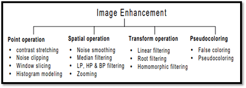
Fig 5 – Image enhancement

Spatial domain enhancement methods

Spatial domain techniques are performed on the image plane, and they directly manipulate the pixel of the image.

Operations are formulated as:

g (x, y) = T [f (x, y)]  

Where g is the output image, f is the input image, and T is an operation

Spatial domain techniques are further divided into 2 categories:

• Point operations (linear operation)
• Spatial operations (non-linear operation)

Frequency domain enhancement methods

Frequency domains enhance an image by following complex linear operators.

1. G (w1, w2) = F (w1, w2) H (w1, w2)  

Image enhancement can also be done through the Gray Level Transformation.

Key takeaway

All Image Processing Techniques focused on gray level transformation as it operates directly on pixels. The gray level image involves 256 levels of gray and in a histogram, the horizontal axis spans from 0 to 255, and the vertical axis depends on the number of pixels in the image.

2.2 Histogram processing

In digital image processing, the histogram is used for the graphical representation of a digital image. A graph is a plot by the number of pixels for each tonal value. Nowadays, image histogram is present in digital cameras. Photographers use them to see the distribution of tones captured.

In a graph, the horizontal axis of the graph is used to represent tonal variations whereas the vertical axis is used to represent the number of pixels in that particular pixel. Black and dark areas are represented on the left side of the horizontal axis, medium grey colour is represented in the middle, and the vertical axis represents the size of the area.

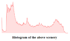
Fig 6 – Histogram

Applications of Histograms

1. In digital image processing, histograms are used for simple calculations in software.
2. It is used to analyze an image. Properties of an image can be predicted by the detailed study of the histogram.
3. The brightness of the image can be adjusted by having the details of its histogram.
4. The contrast of the image can be adjusted according to the need by having details of the x-axis of a histogram.
5. It is used for image equalization. Gray level intensities are expanded along the x-axis to produce a high contrast image.
6. Histograms are used in thresholding as it improves the appearance of the image.
7. If we have an input and output histogram of an image, we can determine which type of transformation is applied in the algorithm.

Histogram Processing Techniques

Histogram Sliding

In Histogram sliding, the complete histogram is shifted towards rightwards or leftwards. When a histogram is shifted towards the right or left, clear changes are seen in the brightness of the image. The brightness of the image is defined by the intensity of light that is emitted by a particular light source.

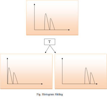
Fig 7 – Histogram sliding

Histogram Stretching

In histogram stretching, the contrast of an image is increased. The contrast of an image is defined between the maximum and minimum value of pixel intensity.

If we want to increase the contrast of an image, the histogram of that image will be fully stretched and covered the dynamic range of the histogram.

From the histogram of an image, we can check that the image has low or high contrast.

Fig 8 – low or high contrast

Histogram Equalization

Histogram equalization is used for equalizing all the pixel values of an image. Transformation is done in such a way that a uniformly flattened histogram is produced.

Histogram equalization increases the dynamic range of pixel values and makes an equal count of pixels at each level which produces a flat histogram with high contrast image.

While stretching histogram, the shape of the histogram remains the same whereas in Histogram equalization, the shape of histogram changes and it generates only one image.

Fig 9 – Transformation

Key takeaway

In digital image processing, the histogram is used for the graphical representation of a digital image. A graph is a plot by the number of pixels for each tonal value. Nowadays, image histogram is present in digital cameras. Photographers use them to see the distribution of tones captured.

In a graph, the horizontal axis of the graph is used to represent tonal variations whereas the vertical axis is used to represent the number of pixels in that particular pixel. Black and dark areas are represented on the left side of the horizontal axis, medium grey color is represented in the middle, and the vertical axis represents the size of the area.

2.3 Basics of Spatial Filtering, Smoothing and Sharpening Spatial Filtering

The spatial Filtering technique is used directly on pixels of an image. Mask is usually considered to be added in size so that it has a specific center pixel. This mask is moved on the image such that the center of the mask traverses all image pixels.

Classification based on linearity:

There are two types:

1. Linear Spatial Filter

2. Non-linear Spatial Filter

General Classification:

Smoothing Spatial Filter: Smoothing filter is used for blurring and noise reduction in the image. Blurring is pre-processing steps for the removal of small details and Noise Reduction is accomplished by blurring.

Types of Smoothing Spatial Filter:

1. Linear Filter (Mean Filter)

2. Order Statistics (Non-linear) filter

These are explained below.

1. Mean Filter:

Linear spatial filter is simply the average of the pixels contained in the neighborhood of the filter mask. The idea is replacing the value of every pixel in an image with the average of the grey levels in the neighborhood defined by the filter mask.

Types of Mean filter:

• (i) Averaging filter: It is used in the reduction of the detail in the image. All coefficients are equal.
• (ii) Weighted averaging filter: In this, pixels are multiplied by different coefficients. The Center pixel is multiplied by a higher value than an average filter.

2.     Order Statistics Filter:

It is based on the ordering of the pixels contained in the image area encompassed by the filter. It replaces the value of the center pixel with the value determined by the ranking result. Edges are better preserved in this filtering.

Types of Order statistics filter:

• (i) Minimum filter: 0th percentile filter is the minimum filter. The value of the center is replaced by the smallest value in the window.
• (ii) Maximum filter: 100th percentile filter is the maximum filter. The value of the center is replaced by the largest value in the window.
• (iii) Median filter: Each pixel in the image is considered. First neighboring pixels are sorted and the original values of the pixel are replaced by the median of the list.

Sharpening Spatial Filter: It is also known as a derivative filter. The purpose of the sharpening spatial filter is just the opposite of the smoothing spatial filter. Its main focus is on the removal of blurring and highlight the edges. It is based on the first and second-order derivatives.

First-order derivative:

• Must be zero in flat segments.
• Must be non-zero at the onset of a grey level step.
• Must be non-zero along ramps.

First order derivative in 1-D is given by:

f' = f(x+1) - f(x)

Second order derivative:

• Must be zero in flat areas.
• Must be zero at the onset and end of a ramp.
• Must be zero along ramps.

Second order derivative in 1-D is given by:

f'' = f(x+1) + f(x-1) - 2f(x)

Key takeaway

The spatial Filtering technique is used directly on pixels of an image. Mask is usually considered to be added in size so that it has a specific center pixel. This mask is moved on the image such that the center of the mask traverses all image pixels.

Classification based on linearity:

There are two types:

1. Linear Spatial Filter

2. Non-linear Spatial Filter

2.4 Frequency Domain: Introduction to Fourier Transform

In the frequency domain, a digital image is converted from spatial domain to frequency domain. In the frequency domain, image filtering is used for image enhancement for a specific application. A Fast Fourier transformation is a tool of the frequency domain used to convert the spatial domain to the frequency domain. For smoothing and image, the low filter is implemented and for sharpening an image, a high pass filter is implemented. When both the filters are implemented, it is analyzed for the ideal filter, Butterworth filter, and Gaussian filter.

The frequency domain is a space that is defined by the Fourier transform. Fourier transform has a very wide application in image processing. Frequency domain analysis is used to indicate how signal energy can be distributed in a range of frequencies.

The basic principle of frequency domain analysis in image filtering is to computer 2D discrete Fourier transform of the image.

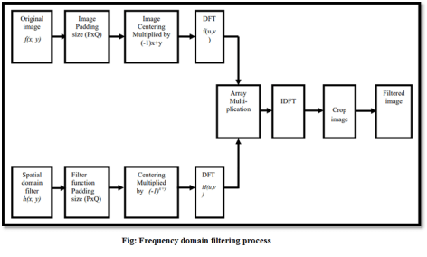
Fig 10 – Frequency domain filtering process

Fourier Series and Transform

Fourier Series

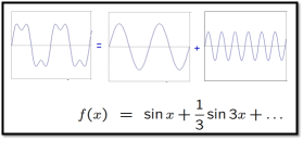
Fourier series is a state in which periodic signals are represented by summing up sines and cosines and multiplied with a certain weight. The periodic signals are further broken down into more signals with some properties which are listed below:

1. Broken signals are sines and cosines.
2. New signals are harmonics of each other.

Fourier series analysis of a step edge:

Fourier decomposition

Fourier Series

Example:

Fourier Transformation

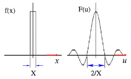
Fourier transformation is a tool for image processing. It is used for decomposing an image into sine and cosine components. The input image is a spatial domain and the output is represented in the Fourier or frequency domain. Fourier transformation is used in a wide range of applications such as image filtering, image compression. Image analysis and image reconstruction etc.

The formula for Fourier transformation:

Example:

Key takeaway

In the frequency domain, a digital image is converted from spatial domain to frequency domain. In the frequency domain, image filtering is used for image enhancement for a specific application. A Fast Fourier transformation is a tool of the frequency domain used to convert the spatial domain to the frequency domain. For smoothing an image, a low filter is implemented and for sharpening an image, a high pass filter is implemented. When both the filters are implemented, it is analyzed for the ideal filter, Butterworth filter, and Gaussian filter.

2.5 Smoothing and sharpening frequency domain filters, Ideal, Butterworth, and Gaussian filters

Lowpass filter (smoothing)

A low pass filter is used to pass low-frequency signals. The strength of the signal is reduced and frequencies that are passed are higher than the cut-off frequency. The amount of strength reduced for each frequency depends on the design of the filter. Smoothing is a low pass operation in the frequency domain.

Following are some lowpass filters:

1. Ideal Lowpass Filters

The ideal lowpass filter is used to cut off all the high-frequency components of Fourier transformation.

Below is the transfer function of an ideal lowpass filter.

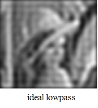
2. Butterworth Lowpass Filters

Butterworth Lowpass Filter is used to remove high-frequency noise with very minimal loss of signal components.

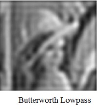
3. Gaussian Lowpass Filters

The transfer function of Gaussian Lowpass filters is shown below:

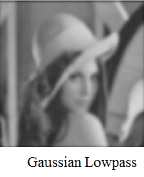
High pass filters (sharpening)

A high pass filter is used for passing high frequencies but the strength of the frequency is lower as compared to the cut-off frequency. Sharpening is a high pass operation in the frequency domain. As a lowpass filter, it also has standard forms such as the Ideal high pass filter, Butterworth high pass filter, Gaussian high pass filter.

Key takeaway

A low pass filter is used to pass low-frequency signals. The strength of the signal is reduced and frequencies that are passed are higher than the cut-off frequency. The amount of strength reduced for each frequency depends on the design of the filter. Smoothing is a low pass operation in the frequency domain.

2.6 Homomorphic filtering

Homomorphic filtering is one such technique for removing multiplicative noise that has certain characteristics.

Homomorphic filtering is most commonly used for correcting non-uniform illumination in images. The illumination-reflectance model of image formation says that the intensity at any pixel, which is the amount of light reflected by a point on the object, is the product of the illumination of the scene and the reflectance of the object(s) in the scene, i.e.,

I (x, y) =L (x, y) R (x, y)

Where I

Is the image, L is scene illumination, and R is the scene reflectance. Reflectance R arises from the properties of the scene objects themselves, but illumination L results from the lighting conditions at the time of image capture. To compensate for the non-uniform illumination, the key is to remove the illumination component L and keep only the reflectance component R

If we consider illumination as the noise signal (which we want to remove), this model is similar to the multiplicative noise model shown earlier.

Illumination typically varies slowly across the image as compared to reflectance which can change quite abruptly at object edges. This difference is the key to separating the illumination component from the reflectance component. In homomorphic filtering, we first transform the multiplicative components into additive components by moving to the log domain.

Ln (I (x, y)) =ln (L (x, y) R (x, y))

Ln (I (x, y)) =ln (L (x, y)) +ln (R (x, y))

Then we use a high-pass filter in the log domain to remove the low-frequency illumination component while preserving the high-frequency reflectance component. The basic steps in homomorphic filtering are shown in the diagram below:

For a working example, I will use an image from the Image Processing Toolbox.

I = imread('AT3_1m4_01.tif');

Imshow(I)

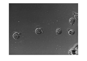
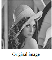
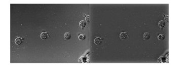
In this image, the background illumination changes gradually from the top-left 1corner to the bottom-right corner of the image. Let's use homomorphic filtering to correct this non-uniform illumination.

The first step is to convert the input image to the log domain. Before that, we will also convert the image to a floating-point type.

I = im2double(I);

I = log (1 + I);

The next step is to do high-pass filtering. We can do high-pass filtering in either the spatial or the spectral domain. Although they are both exactly equivalent, each domain offers some practical advantages of its own. We will do both ways. Let's start with frequency-domain filtering. In the frequency domain the homomorphic filtering process looks like this:

First, we will construct a frequency-domain high-pass filter. There are different types of high-pass filters you can construct, such as Gaussian, Butterworth, and Chebychev filters. We will construct a simple Gaussian high-pass filter directly in the frequency domain. In frequency domain filtering we have to care about the wraparound error which comes from the fact that Discrete Fourier Transform treats a finite-length signal (such as the image) as an infinite-length periodic signal where the original finite-length signal represents one period of the signal. Therefore, there is interference from the non-zero parts of the adjacent copies of the signal. To avoid this, we will pad the image with zeros. Consequently, the size of the filter will also increase to match the size of the image.

M = 2*size(I,1) + 1;

N = 2*size(I,2) + 1;

Note that we can make the size of the filter (M, N) even numbers to speed-up the FFT computation, but we will skip that step for the sake of simplicity. Next, we choose a standard deviation for the Gaussian which determines the bandwidth of the low-frequency band that will be filtered out.

Sigma = 10;

And create the high-pass filter...

[X, Y] = meshgrid(1:N,1:M);

CenterX = ceil(N/2);

CenterY = ceil(M/2);

GaussianNumerator = (X - centerX).^2 + (Y - centerY).^2;

H = exp(-gaussianNumerator./(2*sigma.^2));

H = 1 - H;

Couple of things to note here. First, we formulate a low-pass filter and then subtracted it from 1 to get the high-pass filter. Second, this is a centered filter in that the zero-frequency is at the center.

Imshow(H,'InitialMagnification',25)

We can rearrange the filter in the uncentered format using fftshift.

H = fftshift(H);

Next, we high-pass filter the log-transformed image in the frequency domain. First, we compute the FFT of the log-transformed image with zero-padding using the fft2 syntax that allows us to simply pass in the size of the padded image. Then we apply the high-pass filter and compute the inverse-FFT. Finally, we crop the image back to the original unpadded size.

If = fft2(I, M, N);

Iout = real(ifft2(H.*If));

Iout = Iout(1:size(I,1),1:size(I,2));

The last step is to apply the exponential function to invert the log-transform and get the homomorphic filtered image.

Ihmf = exp (Iout) - 1;

Let's look at the original and the homomorphic-filtered images together. The original image is on the left and the filtered image is on the right. If you compare the two images you can see that the gradual change in illumination in the left image has been corrected to a large extent in the image on the right.

Imshowpair(I, Ihmf, 'montage')

Key takeaway

Homomorphic filtering is one such technique for removing multiplicative noise that has certain characteristics.

Homomorphic filtering is most commonly used for correcting non-uniform illumination in images. The illumination-reflectance model of image formation says that the intensity at any pixel, which is the amount of light reflected by a point on the object, is the product of the illumination of the scene and the reflectance of the object(s) in the scene, i.e.,

I (x, y) =L (x, y) R (x, y)

2.7 Color image enhancement

Color spaces are the mathematical representation of a set of colors. There are many color models. Some of them are RGB, CMYK, YIQ, HSV, and HLS, etc. These color spaces are directly related to saturation and brightness. All of these color spaces can be derived using RGB information using devices such as cameras and scanners.

RGB Color Space

RGB stands for Red, Green, and Blue. This color space is widely used in computer graphics. RGB are the main colors from which many colors can be made.

RGB can be represented in the 3-dimensional form:

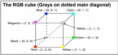
Fig 11 – The RGB cube

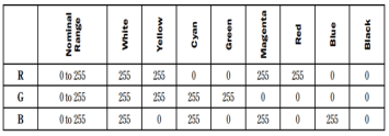
The below table is a 100% RGB color bar that contains values for 100% amplitude, 100% saturated, and video test signal.

CMYK Color Model

CMYK stands for Cyan, Magenta, Yellow, and Black. CMYK color model is used in electrostatic and ink-jet plotters which deposits the pigmentation on paper. In this model, specified color is subtracted from the white light rather than adding blackness. It follows the Cartesian coordinate system and its subset is a unit cube.

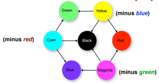
Fig 12 – CMYK Color

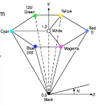
HSV Color Model

HSV stands for Hue, Saturation, and Value (brightness). It is a hexacone subset of the cylindrical coordinate system. The human eye can see 128 different hues, 130 different saturations, and number values between 16 (blue) and 23 (yellow).

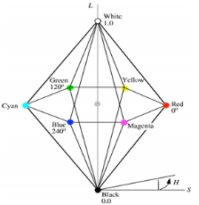
HLS Color Model

HLS stands for Hue Light Saturation. It is a double hexacone subset. The maximum saturation of hue is S= 1 and L= 0.5. It is conceptually easy for people who want to view white as a point.

Key takeaway

Color spaces are the mathematical representation of a set of colors. There are many color models. Some of them are RGB, CMYK, YIQ, HSV, and HLS, etc. These color spaces are directly related to saturation and brightness. All of these color spaces can be derived using RGB information using devices such as cameras and scanners.

References:

1. Rafael C. Gonzalez, Richard E. Woods,  Digital Image Processing Pearson, Third Edition, 2010

2. Anil K. Jain, Fundamentals of Digital Image Processing Pearson, 2002.

3. Kenneth R. Castleman, Digital Image Processing Pearson, 2006.

4. Rafael C. Gonzalez, Richard E. Woods, Steven Eddins, Digital Image Processing using MATLAB Pearson Education, Inc., 2011.

5. D, E. Dudgeon, and RM. Mersereau, Multidimensional Digital Signal Processing Prentice Hall Professional Technical Reference, 1990.

6. William K. Pratt, Digital Image Processing John Wiley, New York, 2002

7. Milan Sonka et al Image processing, analysis and machine vision Brookes/Cole, Vikas Publishing House, 2nd edition, 1999