Unit - 4
Image Segmentation
The concept of edge detection is used to detect the location and presence of edges by making changes in the intensity of an image. Different operations are used in image processing to detect edges. It can detect the variation of grey levels but it quickly gives a response when a noise is detected. In image processing, edge detection is a very important task. Edge detection is the main tool in pattern recognition, image segmentation, and scene analysis. It is a type of filter which is applied to extract the edge points in an image. Sudden changes in an image occur when the edge of an image contour across the brightness of the image.
In image processing, edges are interpreted as a single class of singularity. In a function, the singularity is characterized as discontinuities in which the gradient approaches are infinity.
As we know that the image data is in the discrete form so the edges of the image are defined as the local maxima of the gradient.
Mostly edges exist between objects and objects, primitives and primitives, objects and background. The objects which are reflected are in discontinuous form. Methods of edge detection study to change a single pixel of an image in the gray area.
Edge detection is mostly used for the measurement, detection, and location changes in an image gray. Edges are the basic feature of an image. In an object, the clearest part is the edges and lines. With the help of edges and lines, an object structure is known. That is why extracting the edges is a very important technique in graphics processing and feature extraction.
The basic idea behind edge detection is as follows:
- To highlight local edge operators, use an edge enhancement operator.
- Define the edge strength and set the edge points.
NOTE: edge detection cannot be performed when there are noise and blurring image.
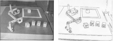
Fig 1 – Edge detection
There are 5 edge detection operators are as follows:
1. Sobel Edge Detection Operator
The Sobel edge detection operator extracts all the edges of an image, without worrying about the directions. The main advantage of the Sobel operator is that it provides a differencing and smoothing effect.
Sobel edge detection operator is implemented as the sum of two-directional edges. And the resulting image is a unidirectional outline in the original image.
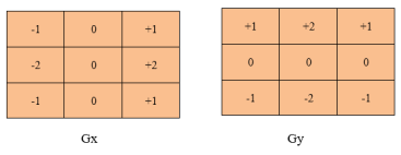
Fig 2 - Sobel edge detection operator
Sobel Edge detection operator consists of 3x3 convolution kernels. Gx is a simple kernel and Gy is rotated by 90°
These Kernels are applied separately to the input image because separate measurements can be produced in each orientation i.e., Gx and Gy.
Following is the gradient magnitude:

As it is much faster to compute an approximate magnitude is computed:

2. Robert's cross operator
Robert's cross operator is used to perform 2-D spatial gradient measurement on an image which is simple and quick to compute. In Robert's cross operator, at each point pixel values represents the absolute magnitude of the input image at that point.
Robert's cross operator consists of 2x2 convolution kernels. Gx is a simple kernel and Gy is rotated by 90o
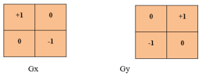
Fig 3 - Robert's cross operator
Following is the gradient magnitude:

As it is much faster to compute an approximate magnitude is computed:

3. Laplacian of Gaussian
The Laplacian of Gaussian is a 2-D isotropic measure of an image. In an image, Laplacian is the highlighted region in which rapid intensity changes, and it is also used for edge detection. The Laplacian is applied to an image which is been smoothed using a Gaussian smoothing filter to reduce the sensitivity of noise. This operator takes a single grey level image as input and produces a single grey level image as output.
Following is the Laplacian L (x, y) of an image that has pixel intensity value I (x, y).

Fig 4 – Example
In Laplacian, the input image is represented as a set of discrete pixels. So discrete convolution kernel which can approximate second derivatives in the definition is found.
3 commonly used kernels are as following:

Fig 5 – 3 commonly used kernels
These are 3 discrete approximations that are used commonly in the Laplacian filter.
Following is 2-D Log function with Gaussian standard deviation:

4. Prewitt operator
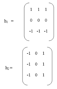
Prewitt operator is a differentiation operator. Prewitt operator is used for calculating the approximate gradient of the image intensity function. In an image, at each point, the Prewitt operator results in a gradient vector or normal vector. In the Prewitt operator, an image is convolved in the horizontal and vertical direction with a small, separable, and integer valued filter. It is inexpensive in terms of computations.
Key takeaway
The concept of edge detection is used to detect the location and presence of edges by making changes in the intensity of an image. Different operations are used in image processing to detect edges. It can detect the variation of grey levels but it quickly gives a response when a noise is detected. In image processing, edge detection is a very important task. Edge detection is the main tool in pattern recognition, image segmentation, and scene analysis. It is a type of filter which is applied to extract the edge points in an image. Sudden changes in an image occur when the edge of an image contour across the brightness of the image.
Hough transform can be used for pixel linking and curve detection. The straight line represented by y=mx+c can be expressed in the polar coordinate system as,
ρ = xcos(θ)+ ysin(θ) …………………...(i)
Where ρ, θ defines a vector from the origin to the nearest point on the straight-line y=mx+c. This vector will be perpendicular from the origin to the nearest point to the line as shown in the below figure.
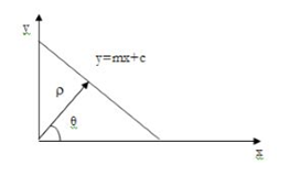
Fig 6 – Straight line
Any line in the x, y plane corresponds to the point in the 2D space defined by the parameter and θ. This the Hough transform of a straight line in the x, y plane is a single point in the ρ, θ space and these points should satisfy the given equation with x1, y1 as constants. Thus, the locus of all such lines in the x, y plane corresponds to the particular sinusoidal curve in the ρ, θ space.
Suppose we have the edge points xi, yi that lies along the straight-line having parameters ρ0, θ0. Each edge point plots to a sinusoidal curve in the ρ, θ space, but these curves must intersect at a point ρ0, θ0. Since this is a line, they all have in common.
For example, considering the equation of a line: y1= ax1+b
Using this equation and varying the values of a and b, infinite lines can pass through this point (x1, y1).
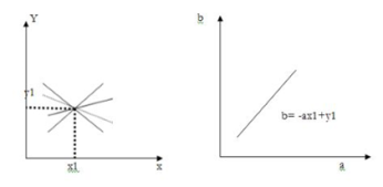
However, if we write the equation as
B= -ax1+y1
And then consider the ab plane instead of xy plane, we get a straight line for a point (xi, yi). This entire line in the ab plane is due to a single point in the xy plane and different values of and b. Now consider another point (x2, y2) in the xy plane. The slope-intercept equation of this line is,
Y2= ax2+ b…………………. (1)
Writing the equation in terms of the ab plane we get,
B= -ax2+y2………………. (2)
This is another line in the ab plane. These two lines will intersect each other somewhere in the ab plane only if they are part of a straight line in the xy plane. The point of intersection in the ab plane is noted as (a’, b’). Using this (a’, b’) in the standard slope-intercept form i.e., y=a’x+b’, we get a line that passes through the points (x1, y1) and (x2, y2) in the xy plane.

Key takeaway
Hough transform can be used for pixel linking and curve detection. The straight line represented by y=mx+c can be expressed in the polar coordinate system as,
ρ = xcos(θ)+ ysin(θ) …………………...(i)
Where ρ, θ defines a vector from the origin to the nearest point on the straight-line y=mx+c. This vector will be perpendicular from the origin to the nearest point to the line
Simple thresholding
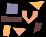
Consider this image, with a series of crudely cut shapes set against a white background. The black outline around the image is not part of the image.
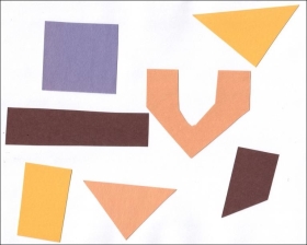
Now suppose we want to select only the shapes from the image. In other words, we want to leave the pixels belonging to the shapes “on,” while turning the rest of the pixels “off,” by setting their color channel values to zeros. The skimage library has several different methods of thresholding. We will start with the simplest version, which involves an important step of human input. Specifically, in this simple, fixed-level thresholding, we have to provide a threshold value, t.
The process works like this. First, we will load the original image, convert it to grayscale, and blur it with one of the methods from the Blurring episode. Then, we will use the > operator to apply the threshold t, a number in the closed range [0.0, 1.0]. Pixels with color values on one side of t will be turned “on,” while pixels with color values on the other side will be turned “off.” To use this function, we have to determine a good value for t. How might we do that? Well, one way is to look at a grayscale histogram of the image. Here is the histogram produced by the GrayscaleHistogram.py program from the Creating Histograms episode, if we run it on the image of the colored shape shown above.
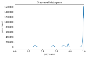
Since the image has a white background, most of the pixels in the image are white. This corresponds nicely to what we see in the histogram: there is a spike near the value of 1.0. If we want to select the shapes and not the background, we want to turn off the white background pixels, while leaving the pixels for the shapes turned on. So, we should choose a value of t somewhere before the large peak and turn pixels above that value “off”.
Here are the first few lines of a Python program to apply simple thresholding to the image, to accomplish this task.
"""
* Python script to demonstrate simple thresholding.
*
* usage: python Threshold.py <filename> <sigma> <threshold>
"""
Import sys
Import numpy as np
Import skimage.color
Import skimage.filters
Import skimage.io
Import skimage.viewer
# get filename, sigma, and threshold value from command line
Filename = sys.argv[1]
Sigma = float(sys.argv[2])
t = float(sys.argv[3])
# read and display the original image
Image = skimage.io.imread(fname=filename)
Viewer = skimage.viewer.ImageViewer(image)
Viewer.show()
This program takes three command-line arguments: the filename of the image to manipulate, the sigma of the Gaussian used during the blurring step (which, if you recall from the Blurring episode, must be a float), and finally, the threshold value t, which should be a float in the closed range [0.0, 1.0]. The program takes the command-line values and stores them in variables named filename, sigma, and t, respectively.
Next, the program reads the original image based on the filename value and displays it.
Now is where the main work of the program takes place.
# blur and grayscale before thresholding
Blur = skimage.color.rgb2gray(image)
Blur = skimage.filters.gaussian(blur, sigma=k)
First, we convert the image to grayscale and then blur it, using the skimage.filter.gaussian() function we learned about in the Blurring episode. We convert the input image to grayscale for easier thresholding.
The fixed-level thresholding is performed using numpy comparison operators.
# perform inverse binary thresholding
Mask = blur < t_rescaled
Here, we want to turn “on” all pixels that have values smaller than the threshold, so we use the less operator < to compare the blurred image blur to the threshold t. The operator returns a binary image, that we capture in the variable mask. It has only one channel, and each of its values is either 0 or 1. Here is a visualization of the binary image created by the thresholding operation. The program used parameters of sigma = 2 and t = 0.8 to produce this image. You can see that the areas where the shapes were in the original area are now white, while the rest of the mask image is black.

We can now apply the mask to the original-colored image as we have learned in the Drawing and Bitwise Operations episode.
# use the mask to select the "interesting" part of the image
Sel = np.zeros_like(image)
Sel[mask] = image[mask]
# display the result
Viewer = skimage.viewer.ImageViewer(sel)
Viewer.view()
What we are left with is only the colored shapes from the original, as shown in this image:
More practice with simple thresholding (15 min)
Now, it is your turn to practice. Suppose we want to use simple thresholding to select only the colored shapes from this image:
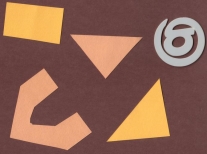
First, use the GrayscaleHistogram.py program in the Desktop/workshops/image-processing/05-creating-histograms directory to examine the grayscale histogram of the more-junk.jpg image, which you will find in the
Desktop/workshops/image-processing/07-thresholding directory.
Via the histogram, what do you think would be a good value for the threshold value, t?
Solution
Now, modify the ThresholdPractice.py program in the
Desktop/workshops/image-processing/07-thresholding directory to turn the pixels above the t value on and turn the pixels below the t value off. To do this, change the comparison operator less < to greater >. Then execute the program on the more-junk.jpg image, using a reasonable value for k and the t value you obtained from the histogram. If everything works as it should, your output should show only the colored shapes on a pure black background.
Solution
Adaptive thresholding
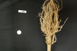
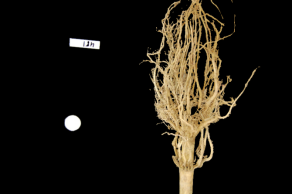
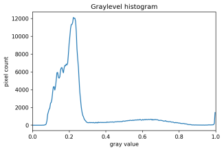
There are also skimage methods to perform adaptive thresholding. The chief advantage of adaptive thresholding is that the value of the threshold, t, is determined automatically for us. One such method, Otsu’s method, is particularly useful for situations where the grayscale histogram of an image has two peaks. Consider this maize root system image, which we have seen before in the Skimage Images episode.
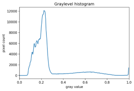
Now, look at the grayscale histogram of this image, as produced by our GrayscaleHistogram.py program from the Creating Histograms episode.
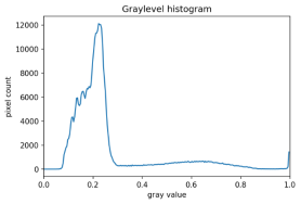
The histogram has a significant peak around 0.2, and a second, albeit smaller peak very near 1.0. Thus, this image is a good candidate for thresholding with Otsu’s method. The mathematical details of how these works are complicated (see the skimage documentation if you are interested), but the outcome is that Otsu’s method finds a threshold value between the two peaks of a grayscale histogram.
The skimage.filters.threshold_otsu() function can be used to determine the adaptive threshold via Otsu’s method. Then numpy comparison operators can be used to apply it as before.
Here is a Python program illustrating how to perform thresholding with Otsu’s method using the skimage.filters.threshold_otsu function. We start by reading and displaying the target image.
"""
* Python script to demonstrate adaptive thresholding using Otsu's method.
*
* usage: python AdaptiveThreshold.py <filename> <sigma>
"""
Import sys
Import numpy as np
Import skimage.color
Import skimage.filters
Import skimage.io
Import skimage.viewer
# get filename and sigma value from command line
Filename = sys.argv[1]
Sigma = float(sys.argv[2])
# read and display the original image
Image = skimage.io.imread(fname=filename)
Viewer = skimage.viewer.ImageViewer(image)
Viewer.show()
The program begins with the now-familiar imports and command-line parameters. Here we only have to get the filename and the sigma of the Gaussian kernel from the command line, since Otsu’s method will automatically determine the thresholding value t. Then, the original image is read and displayed.
Next, a blurred grayscale image is created.
# blur and grayscale before thresholding
Blur = skimage.color.rgb2gray(image)
Blur = skimage.filters.gaussian(image, sigma=sigma)
We determine the threshold via the skimage.filters.threshold_otsu() function:
# perform adaptive thresholding
t = skimage.filters.threshold_otsu(blur)
Mask = blur > t
The function skimage.filters.threshold_otsu() uses Otsu’s method to automatically determine the threshold value based on its inputs grayscale histogram and returns it. Then, we use the comparison operator > for binary the holding. As we have seen before, pixels above the threshold value will be turned on, those below the threshold will be turned off.
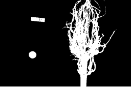
For this root image, and a Gaussian blur with a sigma of 1.0, the computed threshold value is 0.42, and the resulting mask is:
Next, we display the mask and use it to select the foreground
Viewer = skimage.viewer.ImageViewer(mask)
Viewer.show()
# use the mask to select the "interesting" part of the image
Sel = np.zeros_like(image)
Sel[mask] = image[mask]
# display the result
Viewer = skimage.viewer.ImageViewer(sel)
Viewer.show()
Here is the result:
Application: measuring root mass
Let us now turn to an application where we can apply thresholding and other techniques we have learned to this point. Consider these four maize root system images.
Now suppose we are interested in the amount of plant material in each image, and in particular how that amount changes from image to image. Perhaps the images represent the growth of the plant over time, or perhaps the images show four different maize varieties at the same phase of their growth. In any case, the question we would like to answer is, “how much root mass is in each image?” We will construct a Python program to measure this value for a single image, and then create a Bash script to execute the program on each trial image in turn.
Our strategy will be this:
- Read the image, converting it to grayscale as it is read. For this application, we do not need the color image.
- Blur the image.
- Use Otsu’s method of thresholding to create a binary image, where the pixels that were part of the maize plant are white, and everything else is black.
- Save the binary image so it can be examined later.
- Count the white pixels in the binary image, and divide by the number of pixels in the image. This ratio will be a measure of the root mass of the plant in the image.
- Output the name of the image processed and the root mass ratio.
Here is a Python program to implement this root-mass-measuring strategy. Almost all of the code should be familiar, and in fact, it may seem simpler than the code we have worked on thus far because we are not displaying any of the images with this program. Our program here is intended to run and produce its numeric result – a measure of the root mass in the image – without human intervention.
"""
* Python program to determine root mass, as a ratio of pixels in the
* root system to the number of pixels in the entire image.
*
* usage: python RootMass.py <filename> <sigma>
"""
Import sys
Import numpy as np
Import skimage.io
Import skimage.filters
# get filename and sigma value from command line
Filename = sys.argv[1]
Sigma = float(sys.argv[2])
# read the original image, converting to grayscale
Img = skimage.io.imread(fname=filename, as_gray=True)
The program begins with the usual imports and reading of command-line parameters. Then, we read the original image, based on the filename parameter, in grayscale.
Next, the grayscale image is blurred with a Gaussian that is defined by the sigma parameter.
# blur before thresholding
Blur = skimage.filters.gaussian(img, sigma=sigma)
Following that, we create a binary image with Otsu’s method for thresholding, just as we did in the previous section. Since the program is intended to produce numeric output, without a person shepherding it, it does not display any of the images.
# perform adaptive thresholding to produce a binary image
t = skimage.filters.threshold_otsu(blur)
Binary = blur > t
We do, however, want to save the binary images, in case we wish to examine them at a later time. That is what this block of code does:
# save binary image; first find beginning of file extension
Dot = filename.index(".")
Binary_file_name = filename[:dot] + "-binary" + filename[dot:]
Skimage.io.imsave(fname=binary_file_name, arr=skimage.img_as_ubyte(binary))
This code does a little bit of string manipulation to determine the filename to use when the binary image is saved. For example, if the input filename being processed is trial-020.jpg, we want to save the corresponding binary image as trial-020-binary.jpg. To do that, we first determine the index of the dot between the filename and extension – and note that we assume that there is only one dot in the filename! Once we have the location of the dot, we can use slicing to pull apart the filename string, inserting “-binary” in between the end of the original name and the extension. Then, the binary image is saved via a call to the skimage.io.imsave() function. In order to convert from the binary range of 0 and 1 of the mask to a gray level image that can be saved as png, we use the skimage.img_as_ubyte utility function.
Finally, we can examine the code that is the reason this program exists! This block of code determines the root mass ratio in the image:
# determine root mass ratio
RootPixels = np.nonzero(binary)
w = binary.shape[1]
h = binary.shape[0]
Density = rootPixels / (w * h)
# output in format suitable for .csv
Print(filename, density, sep=",")
Recall that we are working with a binary image at this point; every pixel in the image is either zero (black) or 1 (white). We want to count the number of white pixels, which is easily accomplished with a call to the np.count_nonzero function. Then we determine the width and height of the image, via the first and second elements of the image’s shape. Then the density ratio is calculated by dividing the number of white pixels by the total number of pixels in the image. Then, the program prints out the name of the file processed and the corresponding root density.
If we run the program on the trial-016.jpg image, with a sigma value of 1.5, we would execute the program this way:
Python RootMass.py trial-016.jpg 1.5
And the output we would see would be this:
Trial-016.jpg,0.0482436835106383
We have four images to process in this example, and in a real-world scientific situation, there might be dozens, hundreds, or even thousands of images to process. To save us the tedium of running the Python program on each image, we can construct a Bash shell script to run the program multiple times for us. Here is a sample script, which assumes that the images all start with the trial- prefix, and end with the .jpg file extension. The script also assumes that the images, the RootMass.py program, and the script itself are all in the same directory.
#!/bin/bash
# Run the root density mass on all of the root system trail images.
# first, remove existing binary output images
Rm *-binary.jpg
# then, execute the program on all the trail images
For f in trial-*.jpg
Do
Python RootMass.py $f 1.5
Done
The script begins by deleting any prior versions of the binary images. After that, the script uses a for loop to iterate through all of the input images, and execute the RootMass.py on each image with a sigma of 1.5. When we execute the script from the command line, we will see output like this:
Trial-016.jpg,0.0482436835106383
Trial-020.jpg,0.06346941489361702
Trial-216.jpg,0.14073969414893617
Trial-293.jpg,0.13607895611702128
It would probably be wise to save the output of our multiple runs to a file that we can analyze later on. We can do that very easily by redirecting the output stream that would normally appear on the screen to a file. Assuming the shell script is named rootmass.sh, this would do the trick:
Bash rootmass.sh > rootmass.csv
Ignoring more of the images – brainstorming (10 min)
Let us take a closer look at the binary images produced by the proceeding program.
Our root mass ratios include white pixels that are not part of the plant in the image, do they not? The numbered labels and the white circles in each image are preserved during the thresholding, and therefore their pixels are included in our calculations. Those extra pixels might have a slight impact on our root mass ratios, especially the labels since the labels are not the same size in each image. How might we remove the labels and circles before calculating the ratio, so that our results are more accurate? Brainstorm and think about some options, given what we have learned so far.
Solution
Ignoring more of the images – implementation (30 min)
Navigate to the Desktop/workshops/image-processing/07-thresholding directory, and edit the RootMassImproved.py program. This is a copy of the RootMass.py program developed above. Modify the program to apply simple inverse binary thresholding to remove the white circle and label from the image before applying Otsu’s method. Comments in the program show you where you should make your changes.
Solution
Thresholding a bacteria colony image (10 min)
In the Desktop/workshops/image-processing/07-thresholding directory, you will find an image named colonies01.tif; this is one of the images you will be working within the morphometric challenge at the end of the workshop. First, create a grayscale histogram of the image, and determine a threshold value for the image. Then, write a Python program to threshold a grayscale version of the image, leaving the pixels in the bacteria colonies “on,” while turning the rest of the pixels in the image “off.”
Key Points
- Thresholding produces a binary image, where all pixels with intensities above (or below) a threshold value are turned on, while all other pixels are turned off.
- The binary images produced by thresholding are held in two-dimensional NumPy arrays since they have only one color value channel. They are boolean, hence they contain the values 0 (off) and 1 (on).
- Thresholding can be used to create masks that select only the interesting parts of an image, or as the first step before Edge Detection or finding Contours.
Key takeaway
Now suppose we want to select only the shapes from the image. In other words, we want to leave the pixels belonging to the shapes “on,” while turning the rest of the pixels “off,” by setting their color channel values to zeros. The skimage library has several different methods of thresholding. We will start with the simplest version, which involves an important step of human input. Specifically, in this simple, fixed-level thresholding, we have to provide a threshold value, t.
i. The segmentation which is carried out based on similarities in the given image is known as region-based segmentation.
Ii. The regions that are formed using this method have the following properties
a. The sum of all the regions is equal to the whole image.
b. Each region is contiguous and connected
c. A pixel belongs to a single region only, hence there is no overlap of pixels.
d. Each region must satisfy some uniformity condition
e. Two adjacent regions do not have anything in common.
Iii. Region-based segmentation can be carried out in four different ways:
(I) Region Growing
(II) Region Splitting
(III) Region merging
(IV) Split and merge
Each of them is explained below
(I) Region Growing
i. The procedure in which pixels are grouped into larger regions based on some predefined conditions is known as region growing
Ii. The basic approach is to pick a seed point (Starting pixel) and grow regions from this seed pixel
Iii. Let us pick up a random pixel (x1, y1) from the image that needs to be segmented. This pixel is called the seed pixel. The nearest neighbours of (x1, y1) are examined depending on the type of connectivity assumed (4 connectivity or 8 connectivity)
Iv. The neighbouring pixel is accepted in the same region as (x1, y1) if they together satisfy the homogeneity property of a region. That is, both of them satisfy a predefined condition of the region.
v. Once a new pixel say (x2, y2) is accepted as a member of the current region, the neighbours of this new pixel are examined to increase the region further.
Vi. This procedure goes on until no new pixel is accepted. All the pixels of the current region are given a unique label. Now a new seed is chosen and the same procedure is repeated. This procedure is repeated till the time all the pixels are assigned to one group or the other.
(II) Region Splitting
i. In region splitting, we try to satisfy the homogeneity property where similar pixels are grouped.
Ii. If the grey levels present in the region do not satisfy the property, we divide the region into four equal quadrants. If the property is satisfied, we leave the region as it is.
Iii. This is done repeatedly until all the regions satisfy the given property.
Iv. The splitting technique is shown below

v. In the above example, the entire image will be represented by R, this R is the parent node, it is split into four leaf nodes R1, R2, R3, and R4. Of these leaf nodes, only R4 does not contain pixels that satisfy some common property, hence R4 is split into four regions R41, R42, R43 andR44.
Vi. Now if all the pixels in a particular region are satisfying some common property in that region, then splitting is stopped. This is how region splitting works.
(III) Region Merging
i. The region merging method is exactly opposite to the region splitting method
Ii. In this method, we start from the pixel level and consider each of them as a homogeneous region. At any level of merging, we check if four adjacent homogeneous regions are arranged in a 2 x 2 manner, together with satisfying the homogeneity property.
Iii. If the property is satisfied, then the pixels are merged to form a bigger region, otherwise the regions are left as they are.
(IV) Split and Merge
i. Region splitting and region merging were explained above, in region splitting, we start with the whole image and split the image into four quadrants. We continue splitting each quadrant further until all the sub-regions satisfy the predefined homogeneity property.
Ii. In the Region merging each pixel is taken as a small region, we merge small regions into larger regions if they satisfy the homogeneity property.
Iii. If the homogeneous regions are small, the region merging technique is superior and if the regions are large, region splitting is preferred.
Iv. Now, in most applications a combination of both, region splitting and region merging is used.
v. Such a technique where the above combination is used is known as the Split and Merge technique.
Key takeaway
i. The segmentation which is carried out based on similarities in the given image is known as region-based segmentation.
Ii. The regions that are formed using this method have the following properties
. The sum of all the regions is equal to the whole image.
b. Each region is contiguous and connected
c. A pixel belongs to a single region only, hence there is no overlap of pixels.
d. Each region must satisfy some uniformity condition
e. Two adjacent regions do not have anything in common.
Binary images may contain numerous imperfections. In particular, the binary regions produced by simple thresholding are distorted by noise and texture. Morphological image processing pursues the goal of removing these imperfections by accounting for the form and structure of the image. These techniques can be extended to greyscale images.
Basic concepts
Morphological image processing is a collection of non-linear operations related to the shape or morphology of features in an image. According to Wikipedia, morphological operations rely only on the relative ordering of pixel values, not on their numerical values, and therefore are especially suited to the processing of binary images. Morphological operations can also be applied to greyscale images such that their light transfer functions are unknown and therefore their absolute pixel values are of no or minor interest.
Morphological techniques probe an image with a small shape or template called a structuring element. The structuring element is positioned at all possible locations in the image and it is compared with the corresponding neighbourhood of pixels. Some operations test whether the element "fits" within the neighbourhood, while others test whether its "hits" or intersects the neighbourhood:
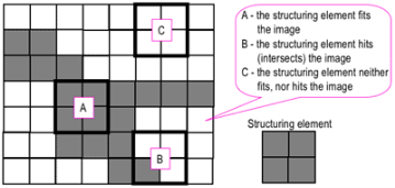
Probing of an image with a structuring element
(White and grey pixels have zero and non-zero values, respectively).
A morphological operation on a binary image creates a new binary image in which the pixel has a non-zero value only if the test is successful at that location in the input image.
The structuring element is a small binary image, i.e., a small matrix of pixels, each with a value of zero or one:
- The matrix dimensions specify the size of the structuring element.
- The pattern of ones and zeros specifies the shape of the structuring element.
- An origin of the structuring element is usually one of its pixels, although generally, the origin can be outside the structuring element.

Examples of simple structuring elements.
A common practice is to have odd dimensions of the structuring matrix and the origin defined as the center of the matrix. Structuring elements play in morphological image processing the same role as convolution kernels in linear image filtering.
When a structuring element is placed in a binary image, each of its pixels is associated with the corresponding pixel of the neighbourhood under the structuring element. The structuring element is said to fit the image if, for each of its pixels set to 1, the corresponding image pixel is also 1. Similarly, a structuring element is said to hit, or intersect, an image if, at least for one of its pixels set to 1 the corresponding image pixel is also 1.

Fitting and hitting of a binary image with structuring elements s1 and s2.
Zero-valued pixels of the structuring element is ignored, i.e., indicate points where the corresponding image value is irrelevant.
Fundamental operations
More formal descriptions and examples of how basic morphological operations work are given in the Hypermedia Image Processing Reference (HIPR) developed by Dr. R. Fisher et al. At the Department of Artificial Intelligence in the University of Edinburgh, Scotland, UK.
Erosion and dilation
The erosion of a binary image f by a structuring element s (denoted f ⊖s) produces a new binary image g = f ⊖s with ones in all locations (x, y) of a structuring element's origin at which that structuring element s fits the input image f, i.e., g (x, y) = 1 is s fits f and 0 otherwise, repeating for all pixel coordinates (x, y).
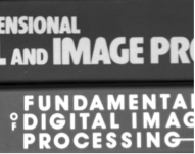


Greyscale image Binary image by thresholding Erosion: a 2×2 square structuring element
Erosion with small (e.g., 2×2 - 5×5) square structuring elements shrink an image by stripping away a layer of pixels from both the inner and outer boundaries of regions. The holes and gaps between different regions become larger, and small details are eliminated:
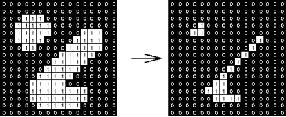
Fig. Erosion: a 3×3 square structuring element
Larger structuring elements have a more pronounced effect, the result of erosion with a large structuring element being similar to the result obtained by iterated erosion using a smaller structuring element of the same shape. If s1 and s2 are a pair of structuring elements identical in shape, with s2 twice the size of s1, then
f ⊖s2 ≈ (f ⊖s1) ⊖s1.
Erosion removes small-scale details from a binary image but simultaneously reduces the size of regions of interest, too. By subtracting the eroded image from the original image, boundaries of each region can be found: b = f − (f ⊖s) where f is an image of the regions, s is a 3×3 structuring element, and b is an image of the region boundaries.
The dilation of an image f by a structuring element s (denoted f ⨁s) produces a new binary image g = f ⨁s with ones in all locations (x, y) of a structuring element's origin at which that structuring element s hits the input image f, i.e., g (x, y) = 1 if s hits f and 0 otherwise, repeating for all pixel coordinates (x, y). Dilation has the opposite effect to erosion -- it adds a layer of pixels to both the inner and outer boundaries of regions.


Binary image Dilation: a 2×2 square structuring element
The holes enclosed by a single region and gaps between different regions become smaller, and small intrusions into boundaries of a region are filled in:
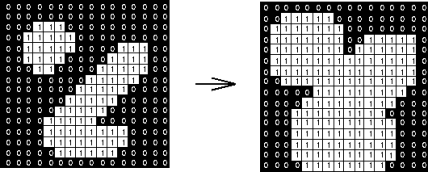
Dilation: a 3×3 square structuring element
Results of dilation or erosion are influenced both by the size and shape of a structuring element. Dilation and erosion are dual operations in that they have opposite effects. Let f c denote the complement of an image f, i.e., the image produced by replacing 1 with 0 and vice versa. Formally, the duality is written as
f ⨁s = f c ⊝srot
Where srot is the structuring element s rotated by 1800. If a structuring element is symmetrical with respect to rotation, then srot does not differ from s. If a binary image is considered to be a collection of connected regions of pixels set to 1 on a background of pixels set to 0, then erosion is the fitting of a structuring element to these regions and dilation is the fitting of a structuring element (rotated if necessary) into the background, followed by inversion of the result.
Compound operations
Many morphological operations are represented as combinations of erosion, dilation, and simple set-theoretic operations such as the complement of a binary image:
f c (x, y) = 1 if f (x, y) = 0, and f c (x, y) = 0 if f (x, y) = 1,
The intersection h = f ∩ g of two binary images f and g:
h (x, y) = 1 if f (x, y) = 1 and g (x, y) = 1, and h (x, y) = 0 otherwise,
And the union h = f ∪ g of two binary images f and g:
h (x, y) = 1 if f (x, y) = 1 or g (x, y) = 1, and h (x, y) = 0 otherwise:

Set operations on binary images: from left to right: a binary image f,
a binary image g, the complement f c of f, the intersection f ∩ g, and the union f ∪ g.
The opening of an image f by a structuring element s (denoted by f o s) is an erosion followed by a dilation:
f o s = (f⊝s) ⨁s


Binary image Opening: a 2×2 square structuring element
The opening is so-called because it can open up a gap between objects connected by a thin bridge of pixels. Any regions that have survived the erosion are restored to their original size by the dilation:
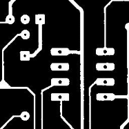
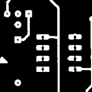
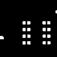
Binary image f f o s (5×5 square) f o s (9×9 square)
Results of opening with a square structuring element
The opening is an idempotent operation: once an image has been opened, subsequent openings with the same structuring element have no further effect on that image:
(f o s) os) = f o s.
The closing of an image f by a structuring element s (denoted by f • s) is a dilation followed by an erosion:
f • s = (f⊕srot) ⊝srot


Binary image Closing: a 2×2 square structuring element
In this case, the dilation and erosion should be performed with a rotated by 1800 structuring element. Typically, the latter is symmetrical, so that the rotated and initial versions of it do not differ.
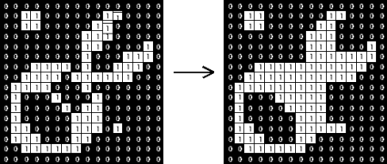
Closing with a 3×3 square structuring element
Closing is so-called because it can fill holes in the regions while keeping the initial region sizes. Like the opening, closing is idempotent: (f • s) • s = f • s, and it is the dual operation of opening (just as the opening is the dual operation of closing):
f • s = (f cos)c; f o s = (f c • s)c.
In other words, closing (opening) of a binary image can be performed by taking the complement of that image, opening (closing) with the structuring element, and taking the complement of the result.
The hit and miss transform allow deriving information on how objects in a binary image are related to their surroundings. The operation requires a matched pair of structuring elements, {s1, s2}, that probe the inside and outside, respectively, of objects in the image:
f ⨁{s1, s2} = (f ⊝s1) ∩ (f c⊝s2).


Binary image Hit and miss transform: an elongated 2×5 structuring element
A pixel belonging to an object is preserved by the hit and miss transform if and only if s1 translated to that pixel fits inside the object AND s2 translated to that pixel fits outside the object. It is assumed that s1 and s2 do not intersect, otherwise, it would be impossible for both fits to occur simultaneously.
It is easier to describe it by considering s1 and s2 as a single structuring element with 1s for pixels of s1 and 0s for pixels of s2; in this case, the hit-and-miss transform assigns 1 to an output pixel only if the object (with the value of 1) and background (with the value of 0) pixels in the structuring element exactly match object (1) and background (0) pixels in the input image. Otherwise, that pixel is set to the background value (0).
The hit and miss transform can be used for detecting specific shapes (spatial arrangements of object and background pixel values) if the two structuring elements present the desired shape, as well as for thinning or thickening of object linear elements.
Morphological filtering
Of a binary image is conducted by considering compound operations like opening and closing as filters. They may act as filters of shape. For example, opening with a disc structuring element smooths corners from the inside, and closing with a disc smooths corners from the outside. But also, these operations can filter out from an image any details that are smaller in size than the structuring element, e.g., opening is filtering the binary image at a scale defined by the size of the structuring element. Only those portions of the image that fit the structuring element are passed by the filter; smaller structures are blocked and excluded from the output image. The size of the structuring element is most important to eliminate noisy details but not to damage objects of interest.
Key takeaway
Binary images may contain numerous imperfections. In particular, the binary regions produced by simple thresholding are distorted by noise and texture. Morphological image processing pursues the goal of removing these imperfections by accounting for the form and structure of the image. These techniques can be extended to greyscale images.
- Visualize an image topographically in 3D
–The two spatial coordinates and the intensity (relief representation).
- Three types of points
–Points belonging to a regional minimum.
–Points at which a drop of water would fall certainly to a regional minimum (catchment basin).
–Points at which the water would be equally likely to fall to more than one regional minimum (crest lines or watershed lines).
- Objective: find the watershed lines.
- Topographic representation.
- The height is proportional to the image intensity.
- Backsides of structures are shaded for better visualization.
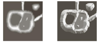
- A hole is punched in each regional minimum and the topography is flooded by water from below through the holes.
- When the rising water is about to merge in catchment basins, a dam is built to prevent merging.
- There will be a stage where only the tops of the dams will be visible.
- These continuous and connected boundaries are the result of the segmentation.
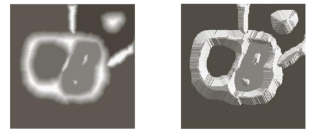
Fig. Topographic representation of the image
- A hole is punched in each regional minimum (dark areas) and the topography is flooded by water (at an equal rate) from below through the holes.
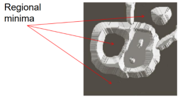
Before flooding
- To prevent water from spilling through the image borders, we consider that the image is surrounded by dams of height greater than the maximum image intensity.

First stage of flooding.
- The water covered areas corresponding to the dark background.

Next stages of flooding.
- The water has risen into the other catchment basin.

- Further flooding. The water has risen into the third catchment basin.

Further flooding.
- The water from the left basin overflowed into the right basin.
- A short dam is constructed to prevent water from merging.
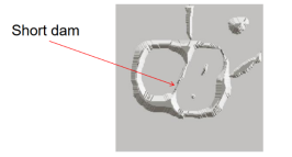
Further flooding.
- The effect is more pronounced.
- The first dam is now longer.
- New dams are created.
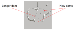
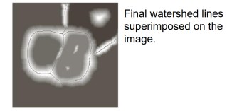
- The process continues until the maximum level of flooding is reached.
- The final dams correspond to the watershed lines which are the result of the segmentation.
- Important: continuous segment boundaries.
- Dams are constructed by morphological dilation.
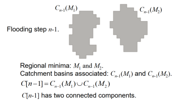
- If we continue flooding, then we will have one connected component.
- This indicates that a dam must be constructed.
- Let q be the merged connected component if we perform flooding a step n.
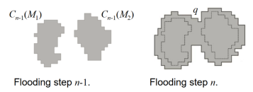
- Each of the connected components is dilated by the SE shown, subject to:
1. The center of the SE has to be contained in q.
2. The dilation cannot be performed on points that would cause the sets to be dilated to merge.
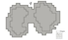
Conditions
1. Center of SE in q.
2. No dilation if merging.
- In the first dilation, condition 1 was satisfied by every point and condition 2 did not apply to any point.
- In the second dilation, several points failed condition 1 while meeting condition 2 (the points in the perimeter which is broken).
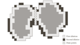
Conditions
1. Center of SE in q.
2. No dilation if merging.
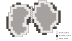
- The only points in q that satisfied both conditions form the 1-pixel thick path.
- This is the dam at step n of the flooding process.
- The points should satisfy both conditions.
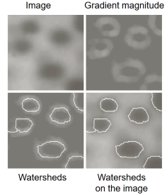
- A common application is the extraction of nearly uniform, blob-like objects from their background.
- For this reason, it is generally applied to the gradient of the image and the catchment basins correspond to the blob-like objects.
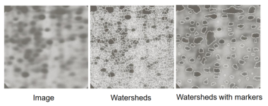
- Noise and local minima lead generally to over-segmentation.
- The result is not useful.
- Solution: limit the number of allowable regions by additional knowledge.
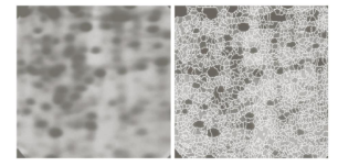
- Markers (connected components):
–internal, associated with the objects
–external, associated with the background.
- Here the problem is a large number of local minima.
- Smoothing may eliminate them.
- Define an internal marker (after smoothing):
- Region surrounded by points of higher altitude.
–They form connected components.
–All points in the connected component have the same intensity.
- After smoothing, the internal markers are shown in light gray.
- The watershed algorithm is applied and the internal markers are the only allowable regional minima.
- The resulting watersheds are the external markers (shown in white).
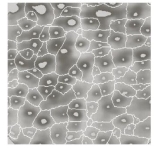
- Each region defined by the external marker has a single internal marker and part of the background.
- The problem is to segment each of these regions into two segments: a single object and background.
- The algorithms we saw in this lecture may be used (including watersheds applied to each region).
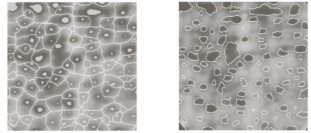
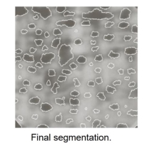
Key takeaway
- Visualize an image topographically in 3D
–The two spatial coordinates and the intensity (relief representation).
- Three types of points
–Points belonging to a regional minimum.
–Points at which a drop of water would fall certainly to a regional minimum (catchment basin).
–Points at which the water would be equally likely to fall to more than one regional minimum (crest lines or watershed lines).
- Objective: find the watershed lines.
- Topographic representation.
- The height is proportional to the image intensity.
Any grayscale image can be viewed as a topographic surface where high intensity denotes peaks and hills while low intensity denotes valleys. You start filling every isolated valley (local minima) with different colored water (labels). As the water rises, depending on the peaks (gradients) nearby, water from different valleys, obviously with different colors will start to merge. To avoid that, you build barriers in the locations where water merges. You continue the work of filling water and building barriers until all the peaks are underwater. Then the barriers you created give you the segmentation result. This is the “philosophy” behind the watershed.
But this approach gives you over segmented result due to noise or any other irregularities in the image. So OpenCV implemented a marker-based watershed algorithm where you specify which are all valley points are to be merged and which are not. It is interactive image segmentation. What we do is to give different labels for our object we know. Label the region which we are sure of being the foreground or object with one color (or intensity), label the region which we are sure of being background or non-object with another color, and finally, the region which we are not sure of anything, label it with 0. That is our marker. Then apply the watershed algorithm. Then our marker will be updated with the labels we gave, and the boundaries of objects will have a value of -1.
Code
Below we will see an example of how to use the Distance Transform along with watershed to segment mutually touching objects.
Consider the coin's image below, the coins are touching each other. Even if your threshold is, it will be touching each other.
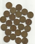
We start by finding an approximate estimate of the coins. For that, we can use the Otsu’s binarization.
Import numpy as np
Import cv2
From matplotlib import pyplot as plt
Img = cv2.imread('coins.png')
Gray = cv2.cvtColor(img,cv2.COLOR_BGR2GRAY)
Ret, thresh =
Cv2.threshold(gray,0,255,cv2.THRESH_BINARY_INV+cv2.THRESH_OTSU)
Result:

Now we need to remove any small white noises in the image. For that, we can use a morphological opening. To remove any small holes in the object, we can use morphological closing. So, now we know for sure that regions near to the center of objects are foreground and region much away from the object are background. The only region we are not sure of is the boundary region of coins.
So, we need to extract the area which we are sure they are coins. Erosion removes the boundary pixels. So, whatever remaining, we can be sure it is a coin. That would work if objects were not touching each other. But since they are touching each other, another good option would be to find the distance transform and apply a proper threshold. Next, we need to find the area in which we are sure they are not coins. For that, we dilate the result. Dilation increases the object boundary to the background. This way, we can make sure whatever region in the background in the result is a background since the boundary region is removed. See the image below.
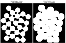
The remaining regions are those which we don’t have any idea, whether it is coins or background. The watershed algorithm should find it. These areas are normally around the boundaries of coins where foreground and background meet (Or even two different coins meet). We call it a border. It can be obtained by subtracting sure_fg area from sure_bg area.
# noise removal
Kernel = np.ones((3,3),np.uint8)
Opening = cv2.morphologyEx(thresh,cv2.MORPH_OPEN,kernel, iterations = 2)
# sure background area
Sure_bg = cv2.dilate(opening,kernel,iterations=3)
# Finding sure foreground area
Dist_transform = cv2.distanceTransform(opening,cv2.DIST_L2,5)
Ret, sure_fg = cv2.threshold(dist_transform,0.7*dist_transform.max(),255,0)
# Finding unknown region
Sure_fg = np.uint8(sure_fg)
Unknown = cv2.subtract(sure_bg,sure_fg)
See the result. In the thresholded image, we get some regions of coins that we are sure of coins and they are detached now. (In some cases, you may be interested in only foreground segmentation, not in separating the mutually touching objects. In that case, you need not use distance transform, just erosion is sufficient. Erosion is just another method to extract sure foreground area, that’s all.)
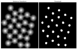
Now we know for sure which are a region of coins, which are background and all. So we create a marker (it is an array of the same size as that of the original image but with int32 data type) and label the regions inside it. The regions we know for sure (whether foreground or background) are labeled with any positive integers, but different integers and the area we don’t know for sure are just left as zero. For this we use cv2.connectedComponents(). It labels the background of the image with 0, then other objects are labeled with integers starting from 1.
But we know that if the background is marked with 0, the watershed will consider it as an unknown area. So, we want to mark it with a different integer. Instead, we will mark the unknown region, defined by unknown, with 0.
# Marker labelling
Ret, markers = cv2.connectedComponents(sure_fg)
# Add one to all labels so that sure background is not 0, but 1
Markers = markers+1
# Now, mark the region of unknown with zero
Markers[unknown==255] = 0
See the result shown in the JET colormap. The dark blue region shows an unknown region. Sure coins are colored with different values. A remaining area which is sure background are shown in lighter blue compared to an unknown region.
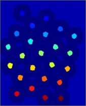
Now our marker is ready. It is time for the final step, apply watershed. Then marker image will be modified. The boundary region will be marked with -1.
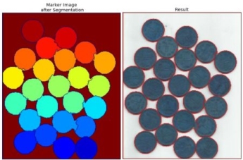
Markers = cv2.watershed(img,markers)
Img[markers == -1] = [255,0,0]
See the result below. For some coins, the region where they touch are segmented properly and for some, they are not.
Key takeaway
Any grayscale image can be viewed as a topographic surface where high intensity denotes peaks and hills while low intensity denotes valleys. You start filling every isolated valley (local minima) with different colored water (labels). As the water rises, depending on the peaks (gradients) nearby, water from different valleys, obviously with different colors will start to merge. To avoid that, you build barriers in the locations where water merges. You continue the work of filling water and building barriers until all the peaks are underwater. Then the barriers you created give you the segmentation result. This is the “philosophy” behind the watershed.
References:
1. Rafael C. Gonzalez, Richard E. Woods, Digital Image Processing Pearson, Third Edition, 2010
2. Anil K. Jain, Fundamentals of Digital Image Processing Pearson, 2002.
3. Kenneth R. Castleman, Digital Image Processing Pearson, 2006.
4. Rafael C. Gonzalez, Richard E. Woods, Steven Eddins, Digital Image Processing using MATLAB Pearson Education, Inc., 2011.
5. D, E. Dudgeon, and RM. Mersereau, Multidimensional Digital Signal Processing Prentice Hall Professional Technical Reference, 1990.
6. William K. Pratt, Digital Image Processing John Wiley, New York, 2002
7. Milan Sonka et al Image processing, analysis and machine vision Brookes/Cole, Vikas Publishing House, 2nd edition, 1999