Unit - 5
Image Compression and Recognition
Data compression is the process of encoding, restructuring, or otherwise modifying data to reduce its size. Fundamentally, it involves re-encoding information using fewer bits than the original representation.
Compression is done by a program that uses functions or an algorithm to effectively discover how to reduce the size of the data. For example, an algorithm might represent a string of bits with a smaller string of bits by using a ‘reference dictionary’ for conversion between them. Another example involves a formula that inserts a reference or pointer to a string of data that the program has already seen. A good example of this often occurs with image compression. When a sequence of colors, like ‘blue, red, red, blue’ is found throughout the image, the formula can turn this data string into a single bit, while still maintaining the underlying information.
Text compression can usually succeed by removing all unnecessary characters, instead of inserting a single character as a reference for a string of repeated characters, then replacing a smaller bit string for a more common bit string. With proper techniques, data compression can effectively lower a text file by 50% or more, greatly reducing its overall size.
For data transmission, compression can be run on the content or the entire transmission. When information is sent or received via the internet, larger files, either on their own or with others, or as part of an archive file, may be transmitted in one of many compressed formats, like ZIP, RAR, 7z, or MP3.
Lossy vs Lossless
Compression is often broken down into two major forms, “lossy” and “lossless”. When choosing between the two methods, it is important to understand their strengths and weaknesses:
- Lossless Compression: Removes bits by locating and removing statistical redundancies. Because of this technique, no information is removed. Lossless compression will often have a smaller compression ratio, with the benefit of not losing any data in the file. This is often very important when needing to maintain absolute quality, as with database information or professional media files. Formats such as FLAC and PNG offer lossless compression options.
- Lossy Compression: Lowers size by deleting unnecessary information, and reducing the complexity of existing information. Lossy compression can achieve much higher compression ratios, at the cost of possible degradation of file quality. JPEG offers lossy compression options, and MP3 is based on lossy compression.
Data Compression Uses
Most businesses today rely on data compression in some major way, especially as the functional quality of data increases, storage capacity concerns have to be resolved. Data compression is one of the major tools that help with this. There some file types that are frequently compressed:
- Audio Compression: Implemented as audio codecs, compression of audio files is necessary to guarantee bandwidth and storage limits aren’t exceeded. Audio compression can be either lossy or lossless, MP3 being the most ubiquitous lossy codec. FLAC is a major lossless encoding format.
- Video Compression: Videos combine image compression with audio compression. There are usually separate codecs for each aspect of a video, which are then wrapped together as a single compression codec. Because of the high data rate required for uncompressed video, most video files are compressed using lossy compression. The most prevalent form of (lossy) video compression is MPEG.
Why Data Compression is Important
The main advantages of compression are reductions in storage hardware, data transmission time, and communication bandwidth. This can result in significant cost savings. Compressed files require significantly less storage capacity than uncompressed files, meaning a significant decrease in expenses for storage. A compressed file also requires less time for transfer while consuming less network bandwidth. This can also help with costs, and also increases productivity.
The main disadvantage of data compression is the increased use of computing resources to apply compression to the relevant data. Because of this, compression vendors prioritize speed and resource efficiency optimizations to minimize the impact of intensive compression tasks.
Key takeaway
Data compression is the process of encoding, restructuring, or otherwise modifying data to reduce its size. Fundamentally, it involves re-encoding information using fewer bits than the original representation.
Compression is done by a program that uses functions or an algorithm to effectively discover how to reduce the size of the data. For example, an algorithm might represent a string of bits with a smaller string of bits by using a ‘reference dictionary’ for conversion between them. Another example involves a formula that inserts a reference or pointer to a string of data that the program has already seen. A good example of this often occurs with image compression. When a sequence of colors, like ‘blue, red, red, blue’ is found throughout the image, the formula can turn this data string into a single bit, while still maintaining the underlying information.
Huffman coding is one of the basic compression methods, that have proven useful in image and video compression standards. When applying the Huffman encoding technique on an Image, the source symbols can be either pixel intensities of the Image or the output of an intensity mapping function.
The first step of the Huffman coding technique is to reduce the input image to an ordered histogram, where the probability of occurrence of a certain pixel intensity value is as
prob_pixel = numpix/totalnum
Where numpix is the number of occurrences of a pixel with a certain intensity value and totalnum is the total number of pixels in the input image.
Let us take an 8 X 8 Image

The pixel intensity values are:
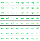
This image contains 46 distinct pixel intensity values, hence we will have 46 unique Huffman code words.
It is evident that not all pixel intensity values may be present in the image and hence will not have a non-zero probability of occurrence.
From here on, the pixel intensity values in the input Image will be addressed as leaf nodes.
Now, there are 2 essential steps to build a Huffman Tree:
- Build a Huffman Tree:
- Combine the two lowest probability leaf nodes into a new node.
- Replace the two leaf nodes with the new node and sort the nodes according to the new probability values.
- Continue the steps (a) and (b) until we get a single node with a probability value of 1.0. We will call this node as root
2. Backtrack from the root, assigning ‘0’ or ‘1’ to each intermediate node, till we reach the leaf nodes
In this example, we will assign ‘0’ to the left child node and ‘1’ to the right one.
Now, let’s look into the implementation:
Step 1:
Read the Image into a 2D array(image)
If the Image is in .bmp format, then the Image can be read into the 2D array.
Int i, j;
Char filename[] = "Input_Image.bmp";
Int data = 0, offset, bpp = 0, width, height;
Long bmpsize = 0, bmpdataoff = 0;
Int** image;
Int temp = 0;
// Reading the BMP File
FILE* image_file;
Image_file = fopen(filename, "rb");
If (image_file == NULL)
{
Printf("Error Opening File!!");
Exit(1);
}
Else
{
// Set file position of the
// stream to the beginning
// Contains file signature
// or ID "BM"
Offset = 0;
// Set offset to 2, which
// contains size of BMP File
Offset = 2;
Fseek(image_file, offset, SEEK_SET);
// Getting size of BMP File
Fread(&bmpsize, 4, 1, image_file);
// Getting offset where the
// pixel array starts
// Since the information
// is at offset 10 from
// the start, as given
// in BMP Header
Offset = 10;
Fseek(image_file, offset, SEEK_SET);
// Bitmap data offset
Fread(&bmpdataoff, 4, 1, image_file);
// Getting height and width of the image
// Width is stored at offset 18 and height
// at offset 22, each of 4 bytes
Fseek(image_file, 18, SEEK_SET);
Fread(&width, 4, 1, image_file);
Fread(&height, 4, 1, image_file);
// Number of bits per pixel
Fseek(image_file, 2, SEEK_CUR);
Fread(&bpp, 2, 1, image_file);
// Setting offset to start of pixel data
Fseek(image_file, bmpdataoff, SEEK_SET);
// Creating Image array
Image = (int**)malloc(height * sizeof(int*));
For (i = 0; i < height; i++)
{
Image[i] = (int*)malloc(width * sizeof(int));
}
// int image[height][width]
// can also be done
// Number of bytes in the
// Image pixel array
Int numbytes = (bmpsize - bmpdataoff) / 3;
// Reading the BMP File
// into Image Array
For (i = 0; i < height; i++)
{
For (j = 0; j < width; j++)
{
Fread(&temp, 3, 1, image_file);
// the Image is a
// 24-bit BMP Image
Temp = temp & 0x0000FF;
Image[i][j] = temp;
}
}
}
Create a Histogram of the pixel intensity values present in the Image
// Creating the Histogram
Int hist[256];
For (i = 0; i < 256; i++)
Hist[i] = 0;
For (i = 0; i < height; i++)
For (j = 0; j < width; j++)
Hist[image[i][j]] += 1;
Find the number of pixel intensity values having the non-zero probability of occurrence
Since the values of pixel intensities range from 0 to 255, and not all pixel intensity values may be present in the image (as evident from the histogram and also the image matrix) and hence will not have a non-zero probability of occurrence. Also, another purpose this step serves, is that the number of pixel intensity values having non-zero probability values will give us the number of leaf nodes in the Image.
// Finding number of
// non-zero occurrences
Int nodes = 0;
For (i = 0; i < 256; i++)
{
If (hist[i] != 0)
Nodes += 1;
}
Calculating the maximum length of Huffman code words
As shown by Y.S.Abu-Mostafa and R.J.McEliece in their paper “Maximal codeword lengths in Huffman codes”, that, If , then in any efficient prefix code for a source whose least probability is p, the longest codeword length is at most K & If , there exists a source whose smallest probability is p, and which has a Huffman code whose longest word has length K. If , there exists such a source for which every optimal code has the longest word of length K.
Here, is the Fibonacci number.
Gallager [1] noted that every Huffman tree is efficient, but it is easy to see more
Generally that every optimal tree is efficient
Fibonacci Series is: 0, 1, 1, 2, 3, 5, 8, 13, 21, 34, 55, 89, 144, …
In our example, lowest probability(p) is 0.015625
Hence,
1/p = 64
For K = 9,
F(K+2) = F(11) = 55
F(K+3) = F(12) = 89
Therefore,
1/F(K+3) < p < 1/F(K+2)
Hence optimal length of code is K=9
// Calculating max length
// of Huffman code word
i = 0;
While ((1 / p) < fib(i))
i++;
Int maxcodelen = i - 3;
// Function for getting Fibonacci
// numbers defined outside main
Int fib(int n)
{
If (n <= 1)
Return n;
Return fib(n - 1) + fib(n - 2);
}
Step 2
Define a struct that will contain the pixel intensity values(pix), their corresponding probabilities(freq), the pointer to the left(*left) and right(*right) child nodes, and also the string array for the Huffman codeword(code).
These structs are defined inside main(), to use the maximum length of code(maxcodelen) to declare the code array field of the struct pixfreq
// Defining Structures pixfreq
Struct pixfreq
{
Int pix;
Float freq;
Struct pixfreq *left, *right;
Char code[maxcodelen];
};
Step 3
Define another Struct that will contain the pixel intensity values(pix), their corresponding probabilities(freq), and an additional field, which will be used for storing the position of newly generated nodes(arrloc).
// Defining Structures huffcode
Struct huffcode
{
Int pix, arrloc;
Float freq;
};
Step 4
Declaring an array of structs. Each element of the array corresponds to a node in the Huffman Tree.
// Declaring structs
Struct pixfreq* pix_freq;
Struct huffcode* huffcodes;
Why use two struct arrays?
Initially, the struct array pix_freq, as well as the struct array huffcodes will only contain the information of all the leaf nodes in the Huffman Tree.
The struct array pix_freq will be used to store all the nodes of the Huffman Tree and the array huffcodes will be used as the updated (and sorted) tree.
Remember that, only huffcodes will be sorted in each iteration, and not pix_freq
The new nodes created by combining two nodes of the lowest frequency, in each iteration, will be appended to the end of the pix_freq array, and also to huffcodes array.
But the array huffcodes will be sorted again according to the probability of occurrence after the new node is added to it.
The position of the new node in the array pix_freq will be stored in the arrloc field of the struct huffcode.
The arrloc field will be used when assigning the pointer to the left and right child of a new node.
Step 4 continued…
Now, if there are N number of leaf nodes, the total number of nodes in the whole Huffman Tree will be equal to 2N-1
And after two nodes are combined and replaced by the new parent node, the number of nodes decreases by 1 at each iteration. Hence, it is sufficient to have a length of nodes for the array huffcodes, which will be used as the updated and sorted Huffman nodes.
Int totalnodes = 2 * nodes - 1;
Pix_freq = (struct pixfreq*)malloc(sizeof(struct pixfreq) * totalnodes);
Huffcodes = (struct huffcode*)malloc(sizeof(struct huffcode) * nodes);
Step 5
Initialize the two arrays pix_freq and huffcodes with information of the leaf nodes.
j = 0;
Int totpix = height * width;
Float tempprob;
For (i = 0; i < 256; i++)
{
If (hist[i] != 0)
{
// pixel intensity value
Huffcodes[j].pix = i;
Pix_freq[j].pix = i;
// location of the node
// in the pix_freq array
Huffcodes[j].arrloc = j;
// probability of occurrence
Tempprob = (float)hist[i] / (float)totpix;
Pix_freq[j].freq = tempprob;
Huffcodes[j].freq = tempprob;
// Declaring the child of
// leaf node as NULL pointer
Pix_freq[j].left = NULL;
Pix_freq[j].right = NULL;
// initializing the code
// word as end of line
Pix_freq[j].code[0] = '\0';
j++;
}
}
Step 6
Sorting the huffcodes array according to the probability of occurrence of the pixel intensity values
Note that, it is necessary to sort the huffcodes array, but not the pix_freq array since we are already storing the location of the pixel values in the arrloc field of the huffcodes array.
// Sorting the histogram
Struct huffcode temphuff;
// Sorting w.r.t probability
// of occurrence
For (i = 0; i < nodes; i++)
{
For (j = i + 1; j < nodes; j++)
{
If (huffcodes[i].freq < huffcodes[j].freq)
{
Temphuff = huffcodes[i];
Huffcodes[i] = huffcodes[j];
Huffcodes[j] = temphuff;
}
}
}
Step 7
Building the Huffman Tree
We start by combining the two nodes with the lowest probabilities of occurrence and then replacing the two nodes with the new node. This process continues until we have a root node. The first parent node formed will be stored at index nodes in the array pix_freq and the subsequent parent nodes obtained will be stored at higher values of the index.
// Building Huffman Tree
Float sumprob;
Int sumpix;
Int n = 0, k = 0;
Int nextnode = nodes;
// Since total number of
// nodes in Huffman Tree
// is 2*nodes-1
While (n < nodes - 1)
{
// Adding the lowest
// two probabilities
Sumprob = huffcodes[nodes - n - 1].freq + huffcodes[nodes - n - 2].freq;
Sumpix = huffcodes[nodes - n - 1].pix + huffcodes[nodes - n - 2].pix;
// Appending to the pix_freq Array
Pix_freq[nextnode].pix = sumpix;
Pix_freq[nextnode].freq = sumprob;
Pix_freq[nextnode].left = &pix_freq[huffcodes[nodes - n - 2].arrloc];
// arrloc points to the location
// of the child node in the
// pix_freq array
Pix_freq[nextnode].right = &pix_freq[huffcodes[nodes - n - 1].arrloc];
Pix_freq[nextnode].code[0] = '\0';
// Using sum of the pixel values as
// new representation for the new node
// since unlike strings, we cannot
// concatenate because the pixel values
// are stored as integers. However, if we
// store the pixel values as strings
// we can use the concatenated string as
// a representation of the new node.
i = 0;
// Sorting and Updating the huffcodes
// array simultaneously New position
// of the combined node
While (sumprob <= huffcodes[i].freq)
i++;
// Inserting the new node in
// the huffcodes array
For (k = nnz; k >= 0; k--)
{
If (k == i)
{
Huffcodes[k].pix = sumpix;
Huffcodes[k].freq = sumprob;
Huffcodes[k].arrloc = nextnode;
}
Else if (k > i)
// Shifting the nodes below
// the new node by 1
// For inserting the new node
// at the updated position k
Huffcodes[k] = huffcodes[k - 1];
}
n += 1;
Nextnode += 1;
}
How does this code work?
Let’s see that by an example:
Initially
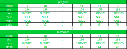
After the First Iteration
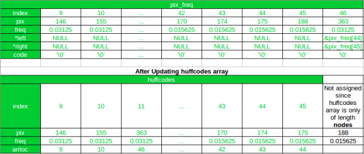
As you can see, after the first iteration, the new node has been appended to the pix_freq array, and its index is 46. And in the huffcode the new node has been added at its new position after sorting, and the arrloc points to the index of the new node in the pix_freq array. Also, notice that all array elements after the new node (at index 11) in huffcodes array have been shifted by 1 and the array element with pixel value 188 gets excluded in the updated array.
Now, in the next(2nd) iteration 170 and 174 will be combined since 175 and 188 have already been combined.
Index of the lowest two nodes in terms of the variable nodes and n is
Left_child_index=(nodes-n-2)
And
Right_child_index=(nodes-n-1)
In 2nd iteration, value of n is 1 (since n starts from 0).
For node having a value of 170
left_child_index=46-1-2=43
For node having value 174
right_child_index=46-1-1=44
Hence, even if 175 remains the last element of the updated array, it will get excluded.
Another thing to notice in this code is that, if in any subsequent iteration, the new node formed in the first iteration is the child of another new node, then the pointer to the new node obtained in the first iteration, can be accessed using the arrloc stored in huffcodes array, as is done in this line of code
Pix_freq[nextnode].right = &pix_freq[huffcodes[nodes - n - 1].arrloc];
Step 8
Backtrack from the root to the leaf nodes to assign code words
Starting from the root, we assign ‘0’ to the left child node and ‘1’ to the right child node.
Now, since we were appending the newly formed nodes to the array pix_freq, hence it is expected that the root will be the last element of the array at index totalnodes-1.
Hence, we start from the last index and iterate over the array, assigning code words to the left and right child nodes, till we reach the first parent node formed at index nodes. We don’t iterate over the leaf nodes since those nodes have NULL pointers as their left and right child.
// Assigning Code through backtracking
Char left = '0';
Char right = '1';
Int index;
For (i = totalnodes - 1; i >= nodes; i--) {
If (pix_freq[i].left != NULL) {
Strconcat(pix_freq[i].left->code, pix_freq[i].code, left);
}
If (pix_freq[i].right != NULL) {
Strconcat(pix_freq[i].right->code, pix_freq[i].code, right);
}
}
Void strconcat(char* str, char* parentcode, char add)
{
Int i = 0;
While (*(parentcode + i) != '\0') {
*(str + i) = *(parentcode + i);
i++;
}
Str[i] = add;
Str[i + 1] = '\0';
}
Final Step
Encode the Image
// Encode the Image
Int pix_val;
// Writing the Huffman encoded
// Image into a text file
FILE* imagehuff = fopen("encoded_image.txt", "wb");
For (r = 0; r < height; r++)
For (c = 0; c < width; c++) {
Pix_val = image[r];
For (i = 0; i < nodes; i++)
If (pix_val == pix_freq[i].pix)
Fprintf(imagehuff, "%s", pix_freq[i].code);
}
Fclose(imagehuff);
// Printing Huffman Codes
Printf("Huffmann Codes::\n\n");
Printf("pixel values -> Code\n\n");
For (i = 0; i < nodes; i++) {
If (snprintf(NULL, 0, "%d", pix_freq[i].pix) == 2)
Printf(" %d -> %s\n", pix_freq[i].pix, pix_freq[i].code);
Else
Printf(" %d -> %s\n", pix_freq[i].pix, pix_freq[i].code);
}
Another important point to note
An average number of bits required to represent each pixel.
// Calculating Average number of bits
Float avgbitnum = 0;
For (i = 0; i < nodes; i++)
Avgbitnum += pix_freq[i].freq * codelen(pix_freq[i].code);
The function codelen calculates the length of codewords OR, the number of bits required to represent the pixel.
Int codelen(char* code)
{
Int l = 0;
While (*(code + l) != '\0')
l++;
Return l;
}
For this specific example image
Average number of bits = 5.343750
The printed results for the example image
pixel values -> Code
72 -> 011001
75 -> 010100
79 -> 110111
83 -> 011010
84 -> 00100
87 -> 011100
89 -> 010000
93 -> 010111
94 -> 00011
96 -> 101010
98 -> 101110
100 -> 000101
102 -> 0001000
103 -> 0001001
105 -> 110110
106 -> 00110
110 -> 110100
114 -> 110101
115 -> 1100
118 -> 011011
119 -> 011000
122 -> 1110
124 -> 011110
125 -> 011111
127 -> 0000
128 -> 011101
130 -> 010010
131 -> 010011
136 -> 00111
138 -> 010001
139 -> 010110
140 -> 1111
142 -> 00101
143 -> 010101
146 -> 10010
148 -> 101011
149 -> 101000
153 -> 101001
155 -> 10011
163 -> 101111
167 -> 101100
169 -> 101101
170 -> 100010
174 -> 100011
175 -> 100000
188 -> 100001
Encoded Image:
0111010101000110011101101010001011010000000101111
00010001101000100100100100010010101011001101110111001
00000001100111101010010101100001111000110110111110010
10110001000000010110000001100001100001110011011110000
10011001101111111000100101111100010100011110000111000
01101001110101111100000111101100001110010010110101000
0111101001100101101001010111
This encoded Image is 342 bits in length, whereas the total number of bits in the original image is 512 bits. (64 pixels each of 8 bits).
Image Compression Code
// C Code for
// Image Compression
#include <stdio.h>
#include <stdlib.h>
// function to calculate word length
Int codelen(char* code)
{
Int l = 0;
While (*(code + l) != '\0')
l++;
Return l;
}
// function to concatenate the words
Void strconcat(char* str, char* parentcode, char add)
{
Int i = 0;
While (*(parentcode + i) != '\0')
{
*(str + i) = *(parentcode + i);
i++;
}
If (add != '2')
{
Str[i] = add;
Str[i + 1] = '\0';
}
Else
Str[i] = '\0';
}
// function to find fibonacci number
Int fib(int n)
{
If (n <= 1)
Return n;
Return fib(n - 1) + fib(n - 2);
}
// Driver code
Int main()
{
Int i, j;
Char filename[] = "Input_Image.bmp";
Int data = 0, offset, bpp = 0, width, height;
Long bmpsize = 0, bmpdataoff = 0;
Int** image;
Int temp = 0;
// Reading the BMP File
FILE* image_file;
Image_file = fopen(filename, "rb");
If (image_file == NULL)
{
Printf("Error Opening File!!");
Exit(1);
}
Else
{
// Set file position of the
// stream to the beginning
// Contains file signature
// or ID "BM"
Offset = 0;
// Set offset to 2, which
// contains size of BMP File
Offset = 2;
Fseek(image_file, offset, SEEK_SET);
// Getting size of BMP File
Fread(&bmpsize, 4, 1, image_file);
// Getting offset where the
// pixel array starts
// Since the information is
// at offset 10 from the start,
// as given in BMP Header
Offset = 10;
Fseek(image_file, offset, SEEK_SET);
// Bitmap data offset
Fread(&bmpdataoff, 4, 1, image_file);
// Getting height and width of the image
// Width is stored at offset 18 and
// height at offset 22, each of 4 bytes
Fseek(image_file, 18, SEEK_SET);
Fread(&width, 4, 1, image_file);
Fread(&height, 4, 1, image_file);
// Number of bits per pixel
Fseek(image_file, 2, SEEK_CUR);
Fread(&bpp, 2, 1, image_file);
// Setting offset to start of pixel data
Fseek(image_file, bmpdataoff, SEEK_SET);
// Creating Image array
Image = (int**)malloc(height * sizeof(int*));
For (i = 0; i < height; i++)
{
Image[i] = (int*)malloc(width * sizeof(int));
}
// int image[height][width]
// can also be done
// Number of bytes in
// the Image pixel array
Int numbytes = (bmpsize - bmpdataoff) / 3;
// Reading the BMP File
// into Image Array
For (i = 0; i < height; i++)
{
For (j = 0; j < width; j++)
{
Fread(&temp, 3, 1, image_file);
// the Image is a
// 24-bit BMP Image
Temp = temp & 0x0000FF;
Image[i][j] = temp;
}
}
}
// Finding the probability
// of occurrence
Int hist[256];
For (i = 0; i < 256; i++)
Hist[i] = 0;
For (i = 0; i < height; i++)
For (j = 0; j < width; j++)
Hist[image[i][j]] += 1;
// Finding number of
// non-zero occurrences
Int nodes = 0;
For (i = 0; i < 256; i++)
If (hist[i] != 0)
Nodes += 1;
// Calculating minimum probability
Float p = 1.0, ptemp;
For (i = 0; i < 256; i++)
{
Ptemp = (hist[i] / (float)(height * width));
If (ptemp > 0 && ptemp <= p)
p = ptemp;
}
// Calculating max length
// of code word
i = 0;
While ((1 / p) > fib(i))
i++;
Int maxcodelen = i - 3;
// Defining Structures pixfreq
Struct pixfreq
{
Int pix, larrloc, rarrloc;
Float freq;
Struct pixfreq *left, *right;
Char code[maxcodelen];
};
// Defining Structures
// huffcode
Struct huffcode
{
Int pix, arrloc;
Float freq;
};
// Declaring structs
Struct pixfreq* pix_freq;
Struct huffcode* huffcodes;
Int totalnodes = 2 * nodes - 1;
Pix_freq = (struct pixfreq*)malloc(sizeof(struct pixfreq) * totalnodes);
Huffcodes = (struct huffcode*)malloc(sizeof(struct huffcode) * nodes);
// Initializing
j = 0;
Int totpix = height * width;
Float tempprob;
For (i = 0; i < 256; i++)
{
If (hist[i] != 0)
{
// pixel intensity value
Huffcodes[j].pix = i;
Pix_freq[j].pix = i;
// location of the node
// in the pix_freq array
Huffcodes[j].arrloc = j;
// probability of occurrence
Tempprob = (float)hist[i] / (float)totpix;
Pix_freq[j].freq = tempprob;
Huffcodes[j].freq = tempprob;
// Declaring the child of leaf
// node as NULL pointer
Pix_freq[j].left = NULL;
Pix_freq[j].right = NULL;
// initializing the code
// word as end of line
Pix_freq[j].code[0] = '\0';
j++;
}
}
// Sorting the histogram
Struct huffcode temphuff;
// Sorting w.r.t probability
// of occurrence
For (i = 0; i < nodes; i++)
{
For (j = i + 1; j < nodes; j++)
{
If (huffcodes[i].freq < huffcodes[j].freq)
{
Temphuff = huffcodes[i];
Huffcodes[i] = huffcodes[j];
Huffcodes[j] = temphuff;
}
}
}
// Building Huffman Tree
Float sumprob;
Int sumpix;
Int n = 0, k = 0;
Int nextnode = nodes;
// Since total number of
// nodes in Huffman Tree
// is 2*nodes-1
While (n < nodes - 1)
{
// Adding the lowest two probabilities
Sumprob = huffcodes[nodes - n - 1].freq + huffcodes[nodes - n - 2].freq;
Sumpix = huffcodes[nodes - n - 1].pix + huffcodes[nodes - n - 2].pix;
// Appending to the pix_freq Array
Pix_freq[nextnode].pix = sumpix;
Pix_freq[nextnode].freq = sumprob;
Pix_freq[nextnode].left = &pix_freq[huffcodes[nodes - n - 2].arrloc];
Pix_freq[nextnode].right = &pix_freq[huffcodes[nodes - n - 1].arrloc];
Pix_freq[nextnode].code[0] = '\0';
i = 0;
// Sorting and Updating the
// huffcodes array simultaneously
// New position of the combined node
While (sumprob <= huffcodes[i].freq)
i++;
// Inserting the new node
// in the huffcodes array
For (k = nodes; k >= 0; k--)
{
If (k == i)
{
Huffcodes[k].pix = sumpix;
Huffcodes[k].freq = sumprob;
Huffcodes[k].arrloc = nextnode;
}
Else if (k > i)
// Shifting the nodes below
// the new node by 1
// For inserting the new node
// at the updated position k
Huffcodes[k] = huffcodes[k - 1];
}
n += 1;
Nextnode += 1;
}
// Assigning Code through
// backtracking
Char left = '0';
Char right = '1';
Int index;
For (i = totalnodes - 1; i >= nodes; i--)
{
If (pix_freq[i].left != NULL)
Strconcat(pix_freq[i].left->code, pix_freq[i].code, left);
If (pix_freq[i].right != NULL)
Strconcat(pix_freq[i].right->code, pix_freq[i].code, right);
}
// Encode the Image
Int pix_val;
Int l;
// Writing the Huffman encoded
// Image into a text file
FILE* imagehuff = fopen("encoded_image.txt", "wb");
For (i = 0; i < height; i++)
For (j = 0; j < width; j++)
{
Pix_val = image[i][j];
For (l = 0; l < nodes; l++)
If (pix_val == pix_freq[l].pix)
Fprintf(imagehuff, "%s", pix_freq[l].code);
}
// Printing Huffman Codes
Printf("Huffmann Codes::\n\n");
Printf("pixel values -> Code\n\n");
For (i = 0; i < nodes; i++) {
If (snprintf(NULL, 0, "%d", pix_freq[i].pix) == 2)
Printf(" %d -> %s\n", pix_freq[i].pix, pix_freq[i].code);
Else
Printf(" %d -> %s\n", pix_freq[i].pix, pix_freq[i].code);
}
// Calculating Average Bit Length
Float avgbitnum = 0;
For (i = 0; i < nodes; i++)
Avgbitnum += pix_freq[i].freq * codelen(pix_freq[i].code);
Printf("Average number of bits:: %f", avgbitnum);
}
Code Compilation and Execution:
First, save the file as “huffman.c“.
For compiling the C file, Open terminal (Ctrl + Alt + T) and enter the following line of code :
Gcc -o huffman huffman.c
For executing the code enter
./huffman
Image Compression Code Output:
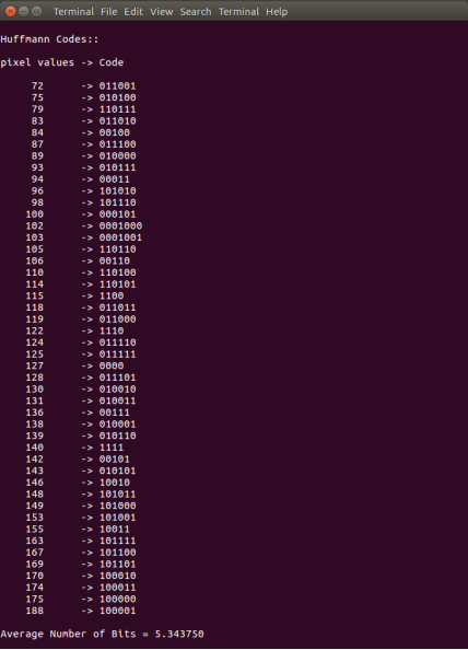
Key takeaway
Huffman coding is one of the basic compression methods, that have proven useful in image and video compression standards. When applying Huffman encoding technique on an Image, the source symbols can be either pixel intensities of the Image or the output of an intensity mapping function.
The first step of Huffman coding technique is to reduce the input image to an ordered histogram, where the probability of occurrence of a certain pixel intensity value is as
prob_pixel = numpix/totalnum
Where numpix is the number of occurrence of a pixel with a certain intensity value and totalnum is the total number of pixels in the input image.
Run-length encoding is a data compression algorithm that is supported by most bitmap file formats, such as TIFF, BMP, and PCX. RLE is suited for compressing any type of data regardless of its information content, but the content of the data will affect the compression ratio achieved by RLE. Although most RLE algorithms cannot achieve the high compression ratios of the more advanced compression methods, RLE is both easy to implement and quick to execute, making it a good alternative to either using a complex compression algorithm or leaving your image data uncompressed.
RLE works by reducing the physical size of a repeating string of characters. This repeating string, called a run, is typically encoded into two bytes. The first byte represents the number of characters in the run and is called the run count. In practice, an encoded run may contain 1 to 128 or 256 characters; the run count usually contains the number of characters minus one (a value in the range of 0 to 127 or 255). The second byte is the value of the character in the run, which is in the range of 0 to 255 and is called the run value.
Uncompressed, a character run of 15 A characters would normally require 15 bytes to store:
AAAAAAAAAAAAAAA
The same string after RLE encoding would require only two bytes:
15A
The 15A code generated to represent the character string is called an RLE packet. Here, the first byte, 15, is the run count and contains the number of repetitions. The second byte, A, is the run value and contains the actual repeated value in the run.
A new packet is generated each time the run character changes, or each time the number of characters in the run exceeds the maximum count. Assume that our 15-character string now contains four different character runs:
AAAAAAbbbXXXXXt
Using run-length encoding this could be compressed into four 2-byte packets:
6A3b5X1t
Thus, after run-length encoding, the 15-byte string would require only eight bytes of data to represent the string, as opposed to the original 15 bytes. In this case, run-length encoding yielded a compression ratio of almost 2 to 1.
Long runs are rare in certain types of data. For example, ASCII plaintext seldom contains long runs. In the previous example, the last run (containing the character t) was only a single character in length; a 1-character run is still a run. Both a run count and a run value must be written for every 2-character run. To encode a run in RLE requires a minimum of two characters' worth of information; therefore, a run of single characters takes more space. For the same reasons, data consisting entirely of 2-character runs remain the same size after RLE encoding.
In our example, encoding the single character at the end as two bytes did not noticeably hurt our compression ratio because there were so many long characters runs in the rest of the data. But observe how RLE encoding doubles the size of the following 14-character string:
Xtmprsqzntwlfb
After RLE encoding, this string becomes:
1X1t1m1p1r1s1q1z1n1t1w1l1f1b
RLE schemes are simple and fast, but their compression efficiency depends on the type of image data being encoded. A black-and-white image that is mostly white, such as the page of a book, will encode very well, due to a large amount of contiguous data that is all the same color. An image with many colors that is very busy in appearance, however, such as a photograph, will not encode very well. This is because the complexity of the image is expressed as a large number of different colors. And because of this complexity, there will be relatively few runs of the same color.
Variants on Run-Length Encoding
There are some variants of run-length encoding. Image data is normally run-length encoded in a sequential process that treats the image data as a 1D stream, rather than as a 2D map of data. In sequential processing, a bitmap is encoded starting at the upper left corner and proceeding from left to right across each scan line (the X-axis) to the bottom right corner of the bitmap. But alternative RLE schemes can also be written to encode data down the length of a bitmap (the Y-axis) along with the columns, to encode a bitmap into 2D tiles, or even to encode pixels on a diagonal in a zig-zag fashion. Odd RLE variants such as this last one might be used in highly specialized applications but are usually quite rare.
![[Graphic: Figure 9-2]](https://glossaread-contain.s3.ap-south-1.amazonaws.com/epub/1657089047_871103.png)
Figure: Run-length encoding variants
Another seldom-encountered RLE variant is a lossy run-length encoding algorithm. RLE algorithms are normally lossless in their operation. However, discarding data during the encoding process, usually by zeroing out one or two least significant bits in each pixel, can increase compression ratios without adversely affecting the appearance of very complex images. This RLE variant works well only with real-world images that contain many subtle variations in pixel values.
Make sure that your RLE encoder always stops at the end of each scan line of bitmap data that is being encoded. There are several benefits to doing so. Encoding only a simple scan line at a time means that only a minimal buffer size is required. Encoding only a simple line at a time also prevents a problem known as cross-coding.
Cross-coding is the merging of scan lines that occurs when the encoding process loses the distinction between the original scan lines. If the data of the individual scan lines are merged by the RLE algorithm, the point where one scan line stopped and another began is lost or, at least, is very hard to detect quickly.
Cross-coding is sometimes done, although we advise against it. It may buy a few extra bytes of data compression, but it complicates the decoding process, adding time cost. For bitmap file formats, this technique defeats the purpose of organizing a bitmap image by scan lines in the first place. Although many file format specifications explicitly state that scan lines should be individually encoded, many applications encode image data as a continuous stream, ignoring scan-line boundaries.
Have you ever encountered an RLE-encoded image file that could be displayed using one application but not using another? Cross-coding is often the reason. To be safe, decoding and display applications must take cross-coding into account and not assume that an encoded run will always stop at the end of a scan line.
When an encoder is encoding an image, an end-of-scan-line marker is placed in the encoded data to inform the decoding software that the end of the scan line has been reached. This marker is usually a unique packet, explicitly defined in the RLE specification, which cannot be confused with any other data packets. End-of-scan-line markers are usually only one byte in length, so they don't adversely contribute to the size of the encoded data.
Encoding scan lines individually has advantages when an application needs to use only part of an image. Let's say that an image contains 512 scan lines, and we need to display only lines 100 to 110. If we did not know where the scan lines started and ended in the encoded image data, our application would have to decode lines 1 through 100 of the image before finding the ten lines it needed. Of course, if the transitions between scan lines were marked with some sort of easily recognizable delimiting marker, the application could simply read through the encoded data, counting markers until it came to the lines it needed. But this approach would be a rather inefficient one.
Another option for locating the starting point of any particular scan line in a block of encoded data is to construct a scan-line table. A scan-line table usually contains one element for every scan line in the image, and each element holds the offset value of its corresponding scan line. To find the first RLE packet of scan line 10, all a decoder needs to do is seek the offset position value stored in the tenth element of the scan-line lookup table. A scan-line table could also hold the number of bytes used to encode each scan line. Using this method, to find the first RLE packet of scan line 10, your decoder would add together the values of the first nine elements of the scan-line table. The first packet for scan line 10 would start at this byte offset from the beginning of the RLE-encoded image data.
Bit-, Byte-, and Pixel-Level RLE Schemes
The basic flow of all RLE algorithms is the same.
![[Graphic: Figure 9-3]](https://glossaread-contain.s3.ap-south-1.amazonaws.com/epub/1657089047_9506855.png)
Figure: Basic run-length encoding flow
The parts of run-length encoding algorithms that differ are the decisions that are made based on the type of data being decoded (such as the length of data runs). RLE schemes used to encode bitmap graphics are usually divided into classes by the type of atomic (that is, most fundamental) elements that they encode. The three classes used by most graphics file formats are bitted -, byte-, and pixel-level RLE.
Bit-level RLE schemes encode runs of multiple bits in a scan line and ignore byte and word boundaries. Only monochrome (black and white), 1-bit images contain a sufficient number of bit runs to make this class of RLE encoding efficient. A typical bit-level RLE scheme encodes runs of one to 128 bits in length in a single-byte packet. The seven least significant bits contain the run count minus one, and the most significant bit contains the value of the bit run, either 0 or 1. A run longer than 128 pixels is split across several RLE-encoded packets.
Byte-level RLE schemes encode runs of identical byte values, ignoring individual bits and word boundaries within a scan line. The most common byte-level RLE scheme encodes runs of bytes into 2-byte packets. The first byte contains the run count of 0 to 255, and the second byte contains the value of the byte run. It is also common to supplement the 2-byte encoding scheme with the ability to store literal, unencoded runs of bytes within the encoded data stream as well.
In such a scheme, the seven least significant bits of the first byte hold the run count minus one, and the most significant bit of the first byte is the indicator of the type of run that follows the run count byte. If the most significant bit is set to 1, it denotes an encoded run. Encoded runs are decoded by reading the run value and repeating it the number of times indicated by the run count. If the most significant bit is set to 0, a literal run is indicated, meaning that the next run count bytes are read literally from the encoded image data. The run count byte then holds a value in the range of 0 to 127 (the run count minus one). Byte-level RLE schemes are good for image data that is stored as one byte per pixel.
Pixel-level RLE schemes are used when two or more consecutive bytes of image data are used to store single-pixel values. At the pixel level, bits are ignored, and bytes are counted only to identify each pixel value. Encoded packet sizes vary depending upon the size of the pixel values being encoded. The number of bits or bytes per pixel is stored in the image file header. A run of image data stored as 3-byte pixel values encodes to a 4-byte packet, with one run-count byte followed by three run-value bytes. The encoding method remains the same as with the byte-oriented RLE.
![[Graphic: Figure 9-4]](https://glossaread-contain.s3.ap-south-1.amazonaws.com/epub/1657089048_0265937.png)
Figure: Bit-, byte-, and pixel-level RLE schemes
It is also possible to employ a literal pixel run encoding by using the most significant bit of the run count as in the byte-level RLE scheme. Remember that the run count in pixel-level RLE schemes is the number of pixels and not the number of bytes in the run.
Earlier in this section, we examined a situation where the string "Xtmprsqzntwlfb" actually doubled in size when compressed using a conventional RLE method. Each 1-character run in the string became two characters in size. How can we avoid this negative compression and still use RLE?
Normally, an RLE method must somehow analyze the uncompressed data stream to determine whether to use a literal pixel run. A stream of data would need to contain many 1- and 2-pixel runs to make using a literal run efficient by encoding all the runs into a single packet. However, there is another method that allows literal runs of pixels to be added to an encoded data stream without being encapsulated into packets.
Consider an RLE scheme that uses three bytes, rather than two, to represent a run. The first byte is a flag value indicating that the following two bytes are part of an encoded packet. The second byte is the count value, and the third byte is the run value. When encoding, if a 1-, 2-, or 3-byte character run is encountered, the character values are written directly to the compressed data stream. Because no additional characters are written, no overhead is incurred.
![[Graphic: Figure 9-5]](https://glossaread-contain.s3.ap-south-1.amazonaws.com/epub/1657089048_1194322.png)
Figure: RLE scheme with three bytes
When decoding, a character is read; if the character is a flag value, the run count and run values are read, expanded, and the resulting run is written to the data stream. If the character read is not a flag value, it is written directly to the uncompressed data stream.
There are two potential drawbacks to this method:
- The minimum useful run-length size is increased from three characters to four. This could affect compression efficiency with some types of data.
- If the unencoded data stream contains a character value equal to the flag value, it must be compressed into a 3-byte encoded packet as a run length of one. This prevents erroneous flag values from occurring in the compressed data stream. If any of these flag value characters are present, poor compression will result. The RLE algorithm must therefore use a flag value that rarely occurs in the uncompressed data stream.
Vertical Replication Packets
Some RLE schemes use other types of encoding packets to increase compression efficiency. One of the most useful of these packets is the repeat scan line packet, also known as the vertical replication packet. This packet does not store any real scan-line data; instead, it just indicates a repeat of the previous scan line. Here's an example of how this works.
Assume that you have an image containing a scan line 640 bytes wide and that all the pixels in the scan line are the same color. It will require 10 bytes to run-length encode it, assuming that up to 128 bytes can be encoded per packet and that each packet is two bytes in size. Let's also assume that the first 100 scan lines of this image are all the same color. At 10 bytes per scan line, that would produce 1000 bytes of run-length encoded data. If we instead used a vertical replication packet that was only one byte in size (possibly a run-length packet with a run count of 0) we would simply run-length encode the first scan line (10 bytes) and follow it with 99 vertical replication packets (99 bytes). The resulting run-length encoded data would then only be 109 bytes in size.
If the vertical replication packet contains a count byte of the number of scan lines to repeat, we would need only one packet with a count value of 99. The resulting 10 bytes of scan-line data packets and two bytes of vertical replication packets would encode the first 100 scan lines of the image, containing 64,000 bytes, as only 12 bytes-- considerable savings.
The figure illustrates 1- and 2-byte vertical replication packets.
![[Graphic: Figure 9-6]](https://glossaread-contain.s3.ap-south-1.amazonaws.com/epub/1657089048_1762924.png)
Figure: RLE scheme with 1- and 2-byte vertical replication packets
Unfortunately, definitions of vertical replication packets are application dependent. At least two common formats, WordPerfect Graphics Metafile (WPG) and GEM Raster (IMG) employ the use of repeat scan line packets to enhance data compression performance. WPG uses a simple 2-byte packet scheme, as previously described. If the first byte of an RLE packet is zero, then this is a vertical replication packet. The next byte that follows indicates the number of times to repeat the previous scan line.
The GEM Raster format is more complicated. The byte sequence, 00h 00h FFh, must appear at the beginning of an encoded scan line to indicate a vertical replication packet. The byte that follows this sequence is the number of times to repeat the previous scan line minus one.
NOTE:
Many of the concepts we have covered in this section are not limited to RLE. All bitmap compression algorithms need to consider the concepts of cross-coding, sequential processing, efficient data encoding based on the data being encoded, and ways to detect and avoid negative compression.
Key takeaway
Run-length encoding is a data compression algorithm that is supported by most bitmap file formats, such as TIFF, BMP, and PCX. RLE is suited for compressing any type of data regardless of its information content, but the content of the data will affect the compression ratio achieved by RLE. Although most RLE algorithms cannot achieve the high compression ratios of the more advanced compression methods, RLE is both easy to implement and quick to execute, making it a good alternative to either using a complex compression algorithm or leaving your image data uncompressed.
The development of multimedia and digital imaging has led to the high quantity of data required to represent modern imagery. This requires large disk space for storage, and a long time for transmission over computer networks, and these two are relatively expensive. These factors prove the need for image compression. Image compression addresses the problem of reducing the amount of space required to represent a digital image yielding a compact representation of an image, and thereby reducing the image storage/transmission time requirements. The key idea here is to remove the redundancy of data presented within an image to reduce its size without affecting the essential information of it. We are concerned with lossless image compression. In this paper, our proposed approach is a mix of some already existing techniques. Our approach works as follows: first, we deal with colors Red, Green, and Blue separately, what comes out of the first step is forward to the second step where the zigzag operation is to rearrange values to be more suitable for preprocessing. At the final, the output from the zigzag enters the shift coding. The experimental results show that the proposed algorithm could achieve an excellent result in a lossless type of compression losing data.
Key takeaway
The development of multimedia and digital imaging has led to the high quantity of data required to represent modern imagery. This requires large disk space for storage, and a long time for transmission over computer networks, and these two are relatively expensive. These factors prove the need for image compression. Image compression addresses the problem of reducing the amount of space required to represent a digital image yielding a compact representation of an image, and thereby reducing the image storage/transmission time requirements.
Arithmetic coding assigns a sequence of bits to a message, a string of symbols. Arithmetic coding can treat the whole symbols in a list or a message as one. Unlike Huffman coding, arithmetic coding doesn’t ́t use a discrete number of bits for each? The number of bits used to encode each symbol varies according to the probability assigned to that symbol. Low probability symbols use many bit, high probability symbols use fewer bits. The main idea behind Arithmetic coding is to assign each symbol an interval. Starting with the interval [0...1), each interval is divided into several subintervals, which its sizes are proportional to the current probability of the corresponding symbols. The subinterval from the coded symbol is then taken as the interval for the next symbol. The output is the interval of the last symbol [1, 3]. The arithmetic coding algorithm is shown in the following.
BEGIN
Low = 0.0; high = 1.0; range = 1.0;
While (symbol != terminator){ get (symbol);
Low = low + range * Range_low(symbol);
High = low + range * Range_high(symbol)
;range = high -low;
}
Output a code so that low <= code < high;
END.
The Figure depicts the flowchart of the arithmetic coding.
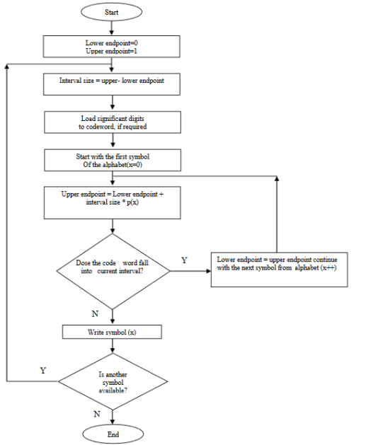
To clarify the arithmetic coding, we explain the previous example using this algorithm. Table 3 depicts the probability and the range of the probability of the symbols between 0 and 1.
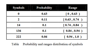
We suppose that the input message consists of the following symbols: 20 0 1360and it starts from left to right. The figure depicts the graphical explanation of the arithmetic algorithm of this message from left to right. As can be seen, the first probability range is 0.63 to 0.74 (Table 3) because the first symbol is 2.
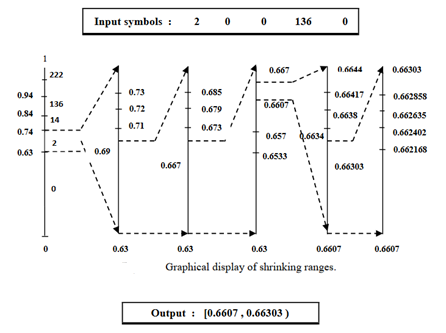
The encoded interval for the mentioned example is [0.6607, 0.66303). A sequence of bits is assigned to a number that is located in this range.
Referring to Figure and considering the discussed example in Figure, we can say that the implementation complexity of arithmetic coding is more than Huffman. We saw this behavior in the programming too.
Key takeaway
Arithmetic coding assigns a sequence of bits to a message, a string of symbols. Arithmetic coding can treat the whole symbols in a list or in a message as one. Unlike Huffman coding, arithmetic coding doesn’t ́t use a discrete number of bits for each? The number of bits used to encode each symbol varies according to the probability assigned to that symbol. Low probability symbols use many bit, high probability symbols use fewer bits. The main idea behind Arithmetic coding is to assign each symbol an interval. Starting with the interval [0...1), each interval is divided into several subintervals, which its sizes are proportional to the current probability of the corresponding symbols.
JPEG and MPEG are the abbreviated names of two standards groups that fall under both the International Organization for Standardization and the International Electrotechnical Commission. JPEG is the Joint Photographic Expert Group, which works on the standards for compression of still digital images. MPEG is the Moving Picture Expert Group, which works on the standards for compression of digital movies. JPEG and MPEG are also the names for the standards published by the respective groups.
Digital images or video are compressed primarily for two reasons: to save storage space for archival, and to save bandwidth in communication, which saves time required to send the data. A compressed digital image or video can be drastically smaller than its original size and saves a great deal of storage space. Upon retrieval, the data can be decompressed to get back the original image or video. When one needs to transmit the data through a channel of a certain bandwidth, the smaller data size also saves transmission time.
There are many different compression algorithms, each with its characteristics and performance. The compressed image or video may be a disk file or a signal in a transmission channel. People need compression standards for interoperability. As long as the data meet the appropriate compression standards, one can display the image or play the video on any system that would observe the same standards.
JPEG
JPEG was proposed in 1991 as a compression standard for digital still images. JPEG compression is lossy, which means that some details may be lost when the image is restored from the compressed data. JPEG compression takes advantage of the way the human eyes work so that people usually do not notice the lost details in the image. With JPEG, one can adjust the amount of loss at compression time by trading image quality for a smaller size of the compressed image.
JPEG is designed for full-color or grayscale images of natural scenes. It works very well with photographic images. JPEG does not work as well on images with sharp edges or artificial scenes such as graphical drawings, text documents, or cartoon pictures.
A few different file formats are used to exchange files with JPEG images. The JPEG File Interchange Format (JFIF) defines a minimum standard necessary to support JPEG, is widely accepted, and is used most often on the personal computer and the Internet. The conventional file name for JPEG images in this format usually has the extension ~.JPG or ~.JPEG (where ~. Represents a file name).
A recent development in the JPEG standard is the JPEG 2000 initiative. JPEG 2000 aims to provide a new image coding system using the latest compression techniques, which are based on the mathematics of wavelets. The effort is expected to find a wide range of applications, from digital cameras to medical imaging.
MPEG
MPEG was first proposed in 1991. It is a family of standards for compressed digital movies and is still evolving. One may think of a digital movie as a sequence of still images displayed one after another at a video rate. However, this approach does not take into consideration the extensive redundancy from frame to frame. MPEG takes advantage of that redundancy to achieve even better compression. A movie also has sound channels to play synchronously with the sequence of images.
The MPEG standards consist of three main parts: video, audio, and systems. The MPEG systems part coordinates between the video and audio parts, as well as coordinating external synchronization for playing.
The MPEG-1 standard was completed in 1993 and was adopted in video CDs. MP3 audio, which is popular on the Internet, is a MPEG-1 standard adopted to handle music in digital audio. It is called MP3 because it is an arrangement for MPEG Audio Layer 3. The MPEG-2 standard was proposed in 1996. It is used as the format for many digital television broadcasting applications and is the basis for digital versatile disks (DVDs), a much more compact version of the video CD with the capacity for full-length movies. The MPEG-4 standard was completed in 1998 and was adopted in 1999. MPEG-4 is designed for transmission over channels with a low bit rate. It is now the popular format for video scripts on the Internet.
These MPEG standards were adopted in a common MPEG format for exchange in disk files. The conventional file name would have the extension ~.MPG or ~.MPEG (where ~ represents a file name). MPEG-7, completed in 2001, is called the Multimedia Content Description Interface. It defines a standard for the textual description of the various multimedia contents, to be arranged in a way that optimizes searching. MPEG-21, called the Multimedia Framework, was started in June 2000. MPEG-21 is intended to integrate the various parts and subsystems into a platform for digital multimedia.
Key takeaway
JPEG and MPEG are the abbreviated names of two standards groups that fall under both the International Organization for Standardization and the International Electrotechnical Commission. JPEG is the Joint Photographic Expert Group, which works on the standards for compression of still digital images. MPEG is the Moving Picture Expert Group, which works on the standards for compression of digital movies. JPEG and MPEG are also the names for the standards published by the respective groups.
• After an image is segmented into regions; the resulting aggregate of segmented pixels is represented & described for further computer processing.
• Representing region involves two choices: in terms of its external characteristics (boundary) in terms of its internal characteristics (pixels comprising the region)
• Above scheme is only part of the task of making data useful to the computer.
• Next task is to Describe the region based on representation.
• Ex. A region may be represented by its boundary & its boundary is described by features such as its length, the orientation of straight-line joining its extreme points & the number of concavities in the boundary.
Q. Which to choose when?
• External representation is chosen when the primary focus is on shape characteristics.
• Internal representation is chosen when the primary focus is on regional properties such as color & texture.
• Sometimes it is necessary to choose both representations.
• Features selected as descriptors should be insensitive to changes in size, translation & rotation.
Representation
• It deals with the compaction of segmented data into representations that facilitate the computation of descriptors.
1) Boundary (Border) Following:
Most of the algorithms require that points in the boundary of a region be ordered in a clockwise (or counterclockwise) direction.
We assume
i) we work with binary images with object and background represented as 1 & 0 respectively.
Ii) Images are padded with borders of 0s to eliminate the possibility of object merging with image border.
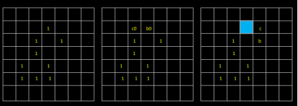
1) Let the starting point b0 be the uppermost, leftmost point in the image. c0 the west neighbor of b0. Examine 8 neighbors of b0 starting at c0 & proceed in a clockwise direction.
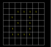
Let b1 denote the first neighbor encountered with value 1 & c1 be background point immediately preceding b1 in the sequence.
2) Let b = b1 & c = c1
3) Let the 8-neighbors of b, starting at c & proceeding in clockwise directions be denoted by n1, n2, …..n8. Find first nk labeled 1.
4) Let b = nk & c = nk-1
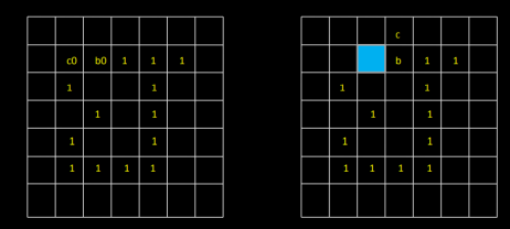
2) Let b = b1 & c = c1
3) Let the 8-neighbors of b, starting at c & proceeding in clockwise directions be denoted by n1, n2, …..n8. Find first nk labeled 1.
4) Let b = nk & c = nk-1
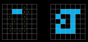
5) Repeat step 3 & 4 until b = b0 & next boundary point found is b1. The sequence of b points found when the algorithm stops constitute the set of ordered boundary points.
The algorithm is also called a Moore boundary tracking algorithm.
2) Chain codes:
They are used to represent a boundary by a connected sequence of straight line segments of specified length & direction.
Typically this representation is based on 4- or 8-connectivity of segments.
The direction of each segment is coded by using a numbering scheme.
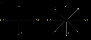
• A boundary code formed as a sequence of such directional numbers is referred to as a Freeman chain code.
• Digital images are acquired & processed in a grid format with equal spacing in x and y directions.
• So a chain code can be generated by following a boundary (say clockwise direction) and assigning a direction to the segments connecting every pair of pixels.
Unacceptable method: (because)
1) Resulting chain tends to be quite long
2) Any small disturbances along the boundary due to noise or imperfect segmentation can cause code changes.
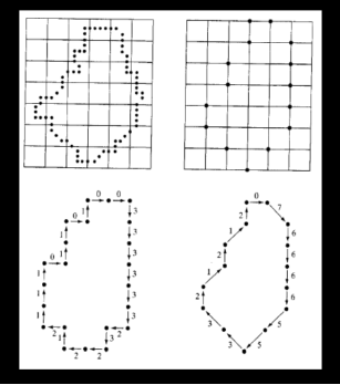
• A solution to this problem is to resample the boundary by selecting a larger grid spacing.
• Then, as the boundary is traversed, a boundary point is assigned to each node of the large grid, depending upon the proximity of the original boundary to that node.
• The re-sampled boundary can now be represented by a 4- or 8-code.
• The accuracy of the resulting code representation depends on the spacing of the sampling grid.
• The chain code of a boundary depends upon the starting point.
• However the code can be normalized:
– We treat the chain code as a circular sequence of direction numbers & redefine the starting point so that the resulting sequence forms an integer of minimum magnitude.
– We can also normalize for rotation by the first difference of the chain code instead of the code itself.
Ex. The first difference between the 4-direction chain code 10103322 is 3133030.
• Considering the circular sequence first element is calculated by subtracting the last and first component. Ex. 33133030
• These normalizations are exact only if the boundaries are invariant to rotation and scale change.
3) Polygon Approximation using Min. Perimeter Polygons:
• A digital boundary can be approximated with arbitrary accuracy by a polygon.
• For a closed boundary, approx becomes exact when no. Of segments of polygon = no. Of points in the boundary.
• Goal of poly. Approx is to capture the essence of the shape in a given boundary using the fewest no. Of segments.
• Min. Perimeter Polygon (MPP):
– An approach for generating an algorithm to compute MPPs is to enclose a boundary by a set of concatenated cells.
– Think boundary as a r u b b e r b a n d.
– As allowed to shrink, it will be constrained by the inner & outer walls of the bounding regions.
• This shrinking produces the shape of a polygon of min. Perimeter.
• Size of cells determines the accuracy of the polygonal approximation.
• In the limit if the size of each cell corresponds to a pixel in the boundary, the error in each cell between the boundary & the MPP approx. At most would be √2d, where d-min possible pixel distance.
• This error can be reduced to half by forcing each cell in poly approx to be centered on its corresponding pixel in the original boundary.
• The objective is to use the largest possible cell size acceptable in a given application.
• Thus, producing MPPs with fewest no. Of vertices.
• The cellular approach reduces the shape of the object enclosed by the original boundary to the area circumscribed by the gray wall.
• Fig. Shows the shape in dark gray.
• Its boundary consists of 4-connected straight line segments.
• If we traverse the boundary in counter clockwise direction.
• Every turn encountered in the transversal will be either a convex (white) or concave(black) vertex, with the angle of the vertex being an interior angle of the 4-connected boundary.
• Every concave vertex has a corresponding mirror vertex in the light gray wall, located diagonally opposite.
• MPP vertices coincide with the convex vertices of the inner wall and mirror concave vertices of the outer wall.
Other Polygonal Approximation Approaches:
• Merging Techniques:
- Techniques based on average error or other criteria have been applied to the problem of polygonal approximation.
- One approach is to merge points along a boundary until the least square error line fit of the points merged so far exceeds a preset threshold.
- When this condition occurs, parameters of the line are stored, the error is set to 0, the procedure is repeated, merging new points along the boundary until the error again exceeds the threshold.
In the end, the intersection of adjacent line segments forms the vertices of the polygon.
Splitting techniques:
One approach to boundary segment splitting is to subdivide a segment successively into two parts until a specified criterion is satisfied.
For ex. A requirement might be that the max. The perpendicular distance from a boundary segment to the line joining its two endpoints not exceeding a preset threshold.
This approach has the advantage of seeking prominent inflection points. For a closed boundary, the best starting points are the two farthest points in the boundary.
Signature:
It is a 1D functional representation of a boundary & may be generated in various ways. One of the simplest is to plot the distance from the centroid to the boundary as a function of angle.
Signatures generated by this method are invariant to translation but they depend on rotation and scaling.
Normalization with respect to rotation can be achieved by finding a way to select the same starting point to generate the signature, regardless of shape’s orientation.
Based on the assumptions of uniformity in scaling wrt. Both axes and that sampling is taken at equal intervals of θ, changes in the size of a shape result in changes in the amplitude values of the corresponding signature.
One way to normalize this is to scale all functions so that they always span the same range of values. e.g [0,1] Main advantage is simplicity but the serious disadvantage is that scaling of the entire function depends upon only two values: maximum & minimum. If the shapes are noisy, an error can occur.
Skeletons: An important approach to represent the structural shape of a plane region is to reduce it to a graph.
The reduction may be accomplished by obtaining the skeleton of the region via the thinning (skeletonizing) algorithm. Ex. Auto inspection of PCB, counting of asbestos fibers in air filters. The Skeleton of a region may be defined as the medial axis transformation (MAT).
MAT of a region R with border B is as follows: For every point p in R, we find its closest neighbor in B. If p has more than such neighbor, it is said to belong to the medial axis (skeleton). ‘prairie fire concept
Implementation involves calculating the distance from every interior point to every boundary point in the region.
Thinning algorithm deals with deleting the boundary points of a region subject to the condition that deleting these points:
1) Does not remove endpoints.
2) Does not break connectivity & 3) Does not cause excessive erosion of the region.
Thinning algorithm: Region points are assumed to have value 1 & background points are assumed to have value 0.

Step 1 flags a contour point for deletion if the following conditions are satisfied:
a) 2 ≤ N(p1) ≤ 6
b) T(p1) = 1
c) p2.p4.p6 = 0
d) p4.p6.p8 = 0
Where N(p1) is the number of nonzero neighbors of p1:
i.e., N(p1) = p2 + p3 + . . . +p8 + p9
Where pi is either 0 or 1.
T(p1) is number of 0-1 transitions in the ordered sequence
p2, p3, . . . p8, p9, p2
In Step 2: conditions a & b remain the same, but conditions c & d are changed to
c’) p2.p4.p8 = 0
d’) p2.p6.p8 = 0 0 0 1 1 p1 0 1 0 1
Step 1 is applied to every border pixel in binary region under consideration If 1 or more of conditions a to d are violated, the value of point in question is not changed.
If all conditions are satisfied, the point is flagged for deletion. But not deleted until all border points have been processed.
This delay prevents the change of structure of data during the execution of the algorithm.
After step 1 has been applied to all border points, those who are flagged are deleted (changed to 0). Step 2 is applied to the resulting data in the exactly same manner as step 1.
Boundary Descriptors:
Simple descriptors: Length: The number of pixels along a boundary gives a rough approximation of its length.
Diameter: Diameter of a boundary is defined as: Diam(B) = max [D(pi,pj)] Where, D – is distance measure & pi, pj – are points on the boundary It is the distance between any two border points on region.
Major axis:
The largest diameter is the major axis Minor axis:
A line perpendicular to the major axis Basic rectangle:
The box consisting of major and minor axes with points intersecting the border forms a basic rectangle.
Eccentricity: Ratio of the major axis to the minor axis. Curvature: It is the rate of change of slope
Shape Numbers: The first difference of a chain coded boundary depends upon the starting point.
The shape number of such a boundary based on 4-directional code is defined as the first difference of the smallest magnitude.
Order n: of a shape is defined as the number of digits in its representation. N is even for a closed boundary.
Key takeaway
- After an image is segmented into regions; the resulting aggregate of segmented pixels is represented & described for further computer processing.
- Representing region involves two choices: in terms of its external characteristics (boundary) in terms of its internal characteristics (pixels comprising the region)
- Above scheme is only part of the task of making data useful to the computer.
- Next task is to Describe the region based on representation.
Let x[m] and y[m] be the coordinates of the mth pixel on the boundary of a given 2D shape containing N pixels, a complex number can be formed as,
z[m] = x[m] + jy[m] and the Fourier Descriptor (FD) of this shape is defined as the DFT of: z[m]
Z[k] = DFT[z[m]] = 1/N ∑m=oN-1 z[m]e-j2πmk/ N (k = 0, …, N-1)
FD can be used as a representation of 2D closed shapes independent of their location, scaling, rotation, and starting point. For example, we could use M < N FDs corresponding to the low-frequency components of the boundary to represent the 2D shape. The reconstructed shape based on these FDs approximate the shape without the details (corresponding to the high-frequency components susceptible to noise). However, note that since the Fourier transform is complex, the frequency spectrum has negative frequencies as well as positive frequencies, with the DC component in the middle. Therefore, the inverse transform with M < N components needs to contain both positive and negative terms:
The following figure shows an image of Gumby:

ẑ[m] = ∑k=-M/2M/2 Z[k]ej2πmk/N (m = 0,….., N-1)
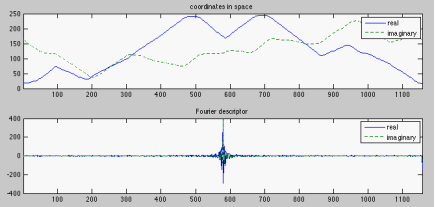
The top part of the following image shows the x (horizontal, red-dashed curve) and y (vertical, blue-continuous curve) coordinates of the N= 1257 pixels on the boundary of the shape, while the bottom part shows the real and imaginary parts of the frequency components, the Fourier descriptors (FD), of the boundary:
The following image shows the reconstruction of Gumby based on the first M < N low-frequency components (excluding the DC). Top: M = 1, 2, 3, and 4; middle: M = 5, 6, 7, and 8; bottom: M = 10, 20, 30, and M = N= 1,257.
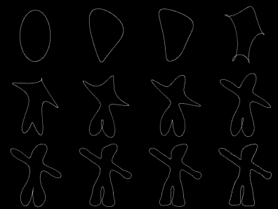
It can be seen that the reconstructed figures using a small percentage of the frequency components are very similar to the actual figure, which can be reconstructed using one hundred percent of the FDs.
Fourier descriptor has the following properties:
- Translation
If the 2D shape is translated by a distance: z0 = x0+ jy0 :
z[m] = z[m] + z0 (m = 0,….., N-1)
: it’s FD becomes
Z[k] : 1/N ∑m=0N-1 z[m] + z0]e-¬¬ j2πmk/N
: 1/N ∑m=0N-1 z[m] e-¬¬ j2πmk/N +1/N ∑m=0N-1 z0 e-¬¬ j2πmk/N
: z[k] + z0 ᵟ [k]
i.e., the translation only affects the DC component Z(0) of the FD.
- Scaling
If the 2D shape is scaled (with respect to origin) by a factor S:
z[m] = S z[m]
Its FD is scaled by the same factor
: Z[k] = S Z[k]
- Rotation
If the 2D shape is rotated about the origin by an angle:
z[m] = z[m]ejᵠ
Its FD is multiplied by the same factor
Z[k] = Z[k] ejᵠ
- Starting Point
If the starting point on the boundary is shifted from 0 to m0:
z[m] = z(m-m0)
By time-shifting theorem, its FD becomes
Z[k] = Z[k] e-j2πm0k/N
Key takeaway
Let x[m] and y[m] be the coordinates of the mth pixel on the boundary of a given 2D shape containing N pixels, a complex number can be formed as
z[m] = x[m] + jy[m], and the Fourier Descriptor (FD) of this shape is defined as the DFT of z[m]:
Z[k] = DFT [z[m]] = 1/N ∑m=0N-1 z[m]e-j2πmk/N (k = 0,….., N-1)
Simple scalar region descriptors
- A large group of shape description techniques is represented by heuristic approaches which yield acceptable results in a description of simple shapes.
- Heuristic region descriptors:
- Area,
- Rectangularity,
- Elongatedness,
- Direction,
- Compactness,
- Etc.
- These descriptors cannot be used for region reconstruction and do not work for more complex shapes.
- Procedures based on region decomposition into smaller and simpler subregions must be applied to describe more complicated regions, then subregions can be described separately using heuristic approaches.
- Simple scalar region descriptors
- The area is given by the number of pixels of which the region consists.
- The real area of each pixel may be taken into consideration to get the real size of a region.
- If an image is represented as a rectangular raster, a simple counting of region pixels will provide its area.
- If the image is represented by a quadtree, then:
Algorithm 6.4: Calculating area in quadtrees
1. Set all region area variiable to zero, and determine the global quadtree depth H; for example, the global quadtree depth is H = 8 for a 256 × 256 image.
2. 2. Search the tree in a systematic way. If a leaf node at a depth h has a non-zero label, process to step (3).
3. 3. Compute:
area[region_label] = area[region_label]+4(H-h)
4. The region area are stored in variables area [region_label]
- The region can also be represented by n polygon vertices
Area = ½ | ∑k=0n-1 (ik jk+1 – ik+1 jk ) |
The sign of the sum represents the polygon orientation.
- If the region is represented by the (anti-clockwise) Freeman chain code the following algorithm provides the area
Algorithm 6.5: Region area calculation from Freeman 4-connectivity chain code representation.
1. Set the region area to zero. Assign the value of the starting point i co-ordinate to the variable.
2. For each element of the chain code (values 0, 1, 2, 3) do
Switch (code) {
Case 0:
Area : = area - vertical_position ;
Break ;
Case 1:
Vartical_position :=vertical_position +1;
Break ;
Case 2 :
Area : = area + vertical_position ;
Break :
Case 3:
- Euler's number
- (sometimes called Genus or the Euler-Poincare characteristic) describes a simple topologically invariant property of the object.
- S is the number of contiguous parts of an object and N is the number of holes in the object (an object can consist of more than one region).
𝛝 = S- N
- Projections
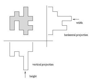
- Horizontal and vertical region projections
Ph(i) = ∑j f(i, j), pv(j) = ∑i f(i, j).
- Eccentricity
- The simplest is the ratio of major and minor axes of an object.
- Elongatedness
- A ratio between the length and width of the region bounding rectangle.
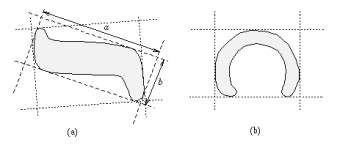
- This criterion cannot succeed in curved regions, for which the evaluation of elongatedness must be based on maximum region thickness.
- Elongatedness can be evaluated as a ratio of the region area and the square of its thickness.
- The maximum region thickness (holes must be filled if present) can be determined as the number d of erosion steps that may be applied before the region totally disappears.
elongatedness = area / (2d)2
- Rectangularity
- Let F_k be the ratio of region area and the area of a bounding rectangle, the rectangle having the direction k. The rectangle direction is turned in discrete steps as before, and rectangularity measured as a maximum of this ratio F_k
Rectangularity = maxk (Fk)
- Direction
- The direction is a property that makes sense in elongated regions only.
- If the region is elongated, the direction is the direction of the longer side of a minimum bounding rectangle.
- If the shape moments are known, the direction \theta can be computed as
ᶿ = ½ tan-1 (2𝛍11 / 𝛍20 – 𝛍02)
- Elongatedness and rectangularity are independent of linear transformations -- translation, rotation, and scaling.
- The direction is independent of all linear transformations which do not include rotation.
- The mutual direction of two rotating objects is rotation invariant.
- Compactness
- Compactness is independent of linear transformations
Compactness = (region_ border_ length)2/ area
- The most compact region in a Euclidean space is a circle.
- Compactness assumes values in the interval [1, infinity) in digital images, if the boundary is defined as an inner boundary while using the outer boundary, compactness assumes values in the interval [16,infty).
- Independence from linear transformations is gained only if an outer boundary representation is used.
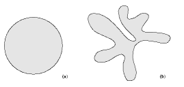
Moments
- Region moment representations interpret a normalized gray level image function as a probability density of a 2D random variable.
- Properties of this random variable can be described using statistical characteristics - moments.
- Assuming that non-zero-pixel values represent regions, moments can be used for binary or gray level region description.
- A moment of order (p+q) is dependent on scaling, translation, rotation, and even on gray level transformations and is given by
Mpq = ʃ-xx ʃ-xx xp yq f(x, y) dx dy
- In digitized images we evaluate sums
mpq = ∑i=-xx ∑j=-xx ipjq f(i, j)
- Where x,y,i,j are the region point co-ordinates (pixel co-ordinates in digitized images).
- Translation invariance can be achieved if we use the central moments
- 𝛍pq = ʃ-xx ʃ-xx (x-xc)p (y-yc)q f(x, y) dx dy
Or in digitized images
𝛍pq = ∑i=-xx ∑j=-xx (i-xc)p (j-yc)q f(i, j)
Where x_c, y_c are the co-ordinates of the region's centroid
xc = m10/m00
yc = m01/m00
- In the binary case, m_00 represents the region area.
- Scale-invariant features can also be found in scaled central moments
ᶯpq = 𝛍pq / (𝛍00)
𝛄= (p+q / 2) +1
𝛍pq = 𝛍pq/(p+q+2)
And normalized unscaled central moments
𝛝pq = 𝛍pq/ (𝛍00)
- Rotation invariance can be achieved if the coordinate system is chosen such that mu_11 = 0.
- A less general form of invariance is given by seven rotation, translation, and scale-invariant moment characteristic
𝝋2 = (𝛝20 – 𝛝02)2 + 4𝛝211
𝝋3 = (𝛝30 – 3𝛝12)2 +(3𝛝21 – 𝛝03)2
𝝋4 = (𝛝30 – 𝛝12)2 +(𝛝21 – 𝛝03)2
𝝋5 = (𝛝30 – 3𝛝12) (𝛝30 + 𝛝12)[ (𝛝30 + 𝛝12)2 - 3(𝛝21 +𝛝03)2] +
(3𝛝21 -𝛝03) (𝛝21 + 𝛝03 ) [3(𝛝30 + 3𝛝12)2 – (𝛝21 + 𝛝03)2]
𝛝6 = (𝛝20 – 𝛝02) [(𝛝30 + 𝛝12)2 – (𝛝21 + 𝛝03)2] + 4𝛝11 (𝛝30 + 𝛝12) (𝛝21 + 𝛝03)
𝛝7 = (3𝛝21- 3𝛝03) (𝛝30 + 𝛝12) [(𝛝30 + 𝛝12)2 – 3(𝛝21 + 𝛝03)2] –
(𝛝30 + 3𝛝12 )( 21 + 𝛝03) [3(𝛝30 + 𝛝12)2 – (𝛝21 + 𝛝03)2]
𝝋1 = 𝛝20 +𝛝02
- While the seven-moment characteristics presented above were shown to be useful, they are only invariant to translation, rotation, and scaling.
- A complete set of four affine moment invariants derived from second-and third-order moments is


- All moment characteristics are dependent on the linear gray level transformations of regions; to describe region shape properties, we work with binary image data (f(i,j)=1 in region pixels) and dependence on the linear gray level transform disappears.
- Moment characteristics can be used in shape description even if the region is represented by its boundary.
- A closed boundary is characterized by an ordered sequence z(i) that represents the Euclidean distance between the centroid and all N boundary pixels of the digitized shape.
- No extra processing is required for shapes having a spiral or concave contours.
- Translation, rotation, and scale-invariant one-dimensional normalized contour sequence moments can be estimated as


- The r-th normalized contour sequence moment and normalized central contour sequence moment are defined as
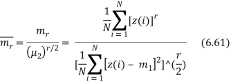
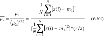
- Less noise-sensitive results can be obtained from the following shape descriptors
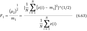
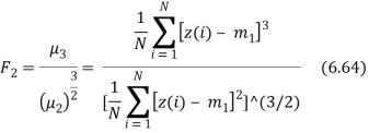
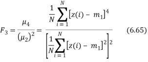

Convex hull
- A region R is convex if and only if for any two points x_1, x_2 from R, the whole line segment defined by its end-points x_1, x_2 is inside the region R.
- The convex hull of a region is the smallest convex region H which satisfies the condition R is a subset of H.
- The convex hull has some special properties in digital data that do not exist in the continuous case. For instance, concave parts can appear and disappear in digital data due to rotation, and therefore the convex hull is not rotation invariant in digital space.
- The convex hull can be used to describe region shape properties and can be used to build a tree structure of region concavity.
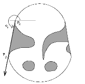
- A discrete convex hull can be defined by the following algorithm which may also be used for convex hull construction.
- This algorithm has complexity O(n^2) and is presented here as an intuitive way of detecting the convex hull.
Algorithm 6.6 : Region convex hull construction
1. Find all pixels of a region R with the minimum row co-ordinate; among them, find the pixel P1 with the minimum column co-ordinate. Assign Pk = P1, v = (0, -1); the vector v represents the direction of the previous line segment of the convex hull.
2. Search the region boundary in an anti-clockwise direction(Algorithm ??) and compute the angle orientation φn for every boundary point Pn which lies after the point P1 (in the direction of boundary search - see Figure 6.26). The angle orientation φn is the angle vector Pk Pn . The point Pn satisfying the condition φq = minn φn is an element (vertex) of the region convex hull.
3. Assign v = PkPnPK = Pq.
4. Repeat steps (2) and (3) until Pk = P1
- More efficient algorithms exist, especially if the object is defined by an ordered sequence of n vertices representing a polygonal boundary of the object.
- If the polygon P is a simple polygon (self-non-intersecting polygon) which is always the case in a polygonal representation of object borders, the convex hull may be found in linear time O(n).
- In the past two decades, many linear-time convex hull detection algorithms have been published, however, more than half of them were later discovered to be incorrect with counter-examples published.
- The simplest correct convex hull algorithm was developed by Melkman and is now discussed further.
- Let the polygon for which the convex hull is to be determined by a simple polygon P = v_1, v_2, ... v_n and let the vertices be processed in this order.
- For any three vertices x,y,z in an ordered sequence, a directional function delta may be evaluated

- The main data structure H is a list of vertices (deque) of polygonal vertices already processed.
- The current contents of H represent the convex hull of the currently processed part of the polygon, and after the detection is completed, the convex hull is stored in this data structure.
- Therefore, H always represents a closed polygonal curve, H={d_b, ... ,d_t} where d_b points to the bottom of the list and d_t points to its top.
- Note that d_b and d_t always refer to the same vertex simultaneously representing the first and the last vertex of the closed polygon.
- Main ideas of the algorithm:
- The first three vertices A, B, C from the sequence P form a triangle (if not collinear) and this triangle represents a convex hull of the first three vertices.
- The next vertex D in the sequence is then tested for being located inside or outside the current convex hull.
- If D is located inside, the current convex hull does not change.
- If D is outside of the current convex hull, it must become a new convex hull vertex, and based on the current convex hull shape, either none, one or several vertices must be removed from the current convex hull.
- This process is repeated for all remaining vertices in the sequence P.

Figure. Convex hull detection: (a) First three vertices A, B, C form a triangle, (b) if the next vertex D is positioned inside the current convex hull ABC, current convex hull does not change, (c) if the next vertex D is outside of the current convex hull, it becomes a new vertex of the new current convex hull ABCDA, (d) in this case, vertex B must be removed from the current convex hull and the current convex hull is ADCA.
- The variable v refers to the input vertex under consideration, and the following operations are defined:
Push v : t:=t+1; dt ----- v
Pop dt : t:= t-1
Insert v : b:= b-1; db---- v
Remove db : b:= b+1
Input v : next vertex is entered from sequence P, if P empty, stop.
- The algorithm is then;
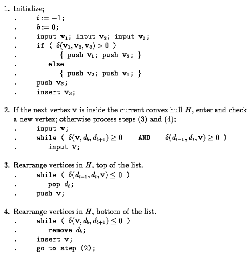
- The algorithm as presented may be difficult to follow, however, a less formal version would be impossible to implement.
- The following example makes the algorithm more understandable.
Let P ={A, B, C, D, E} as shown in Figure 6.29a. The data structure H is created in the first step;

In the second step, vertex D is entered (Figure 6.29b);
δ(D, db, db+1) = δ(D,C,A) = 1 > 0
δ(dt-1, dt, D) = δ(B, C, D) = -1 < 0
Based on the values of the directional function δ, in this case, no other vertex is entered during this step. Step (3) results in the following current convex hull H;
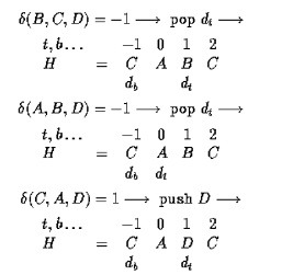
In step (4) - Figure c;

Go to step (2); vertex E is entered - Figure d;

- A new vertex should be entered from P, however, there is no unprocessed vertex in the sequence P, and the convex hull generating process stops.
- The resulting convex hull is defined by the sequence H={d_b, ... ,d_t}={D,C,A,D} which represents a polygon DCAD, always in the clockwise direction.
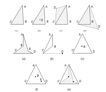
Figure. Example of convex hull detection: (a) The processed region - polygon ABCDEA, (b) vertex D is entered and processed, (c) vertex D becomes a new vertex of the current convex hull ADC, (d) vertex E is entered and processed, E does not become a new vertex of the current convex hull, (e) the resulting convex hull DCAD.
- A region concavity tree is generated recursively during the construction of a convex hull.
- A convex hull of the whole region is constructed first, and convex hulls of concave residua are found next.
- The resulting convex hulls of concave residua of the regions from previous steps are searched until no concave residuum exists.
- The resulting tree is a shape representation of the region.
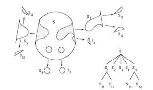
Fig. Concavity tree construction: (a) Convex hull and concave residua, (b) Concavity tree
Graph representation based on region skeleton
- Objects are represented by a planar graph with nodes representing subregions resulting from region decomposition, and region shape is then described by the graph properties.
- There are two general approaches to acquiring a graph of subregions:
- The first one is region thinning leading to the region skeleton, which can be described by a graph.
- The second option starts with the region decomposition into subregions, which are then represented by nodes while arcs represent neighborhood relations of subregions.
- Graphical representation of regions has many advantages; the resulting graphs
- Are translation and rotation invariant; position and rotation can be included in the graph definition
- Are insensitive to small changes in shape
- Are highly invariant with respect to region magnitude
- Generate a representation that is understandable
- Can easily be used to obtain the information-bearing features of the graph
- Are suitable for syntactic recognition
- Graph representation based on region skeleton
- This method corresponds significantly to curving points of a region boundary to graph nodes.
- The main disadvantage of boundary-based description methods is that geometrically close points can be far away from one another when the boundary is described - graphical representation methods overcome this disadvantage.
- The region graph is based on the region skeleton, and the first step is the skeleton construction.
- There are four basic approaches to skeleton construction:
- Thinning - iterative removal of region boundary pixels
- Wave propagation from the boundary
- Detection of local maxima in the distance-transformed image of the region
- Analytical methods
- Most thinning procedures repeatedly remove boundary elements until a pixel set with a maximum thickness of one or two is found. The following algorithm constructs a skeleton of maximum thickness two.
- The steps of this algorithm are illustrated in the next Figure.
- If there are skeleton segments that have a thickness of two, one extra step can be added to reduce those to a thickness of one, although care must be taken not to break the skeleton connectivity.
- Thinning is generally a time-consuming process, although sometimes it is not necessary to look for a skeleton, and one side of a parallel boundary can be used for skeleton-like region representation.
- Mathematical morphology is a powerful tool used to find the region skeleton.
- Thinning procedures often use a medial axis transform to construct a region skeleton.
- Under the medial axis definition, the skeleton is the set of all-region points that have the same minimum distance from the region boundary for at least two separate boundary points.
- Such a skeleton can be constructed using a distance transform which assigns a value to each region pixel representing its (minimum) distance from the region's boundary.
- The skeleton can be determined as a set of pixels whose distance from the region's border is locally maximal.
- Every skeleton element can be accompanied by information about its distance from the boundary -- this gives the potential to reconstruct a region as an envelope curve of circles with center points at skeleton elements and radii corresponding to the stored distance values.
- Small changes in the boundary may cause serious changes in the skeleton.
- This sensitivity can be removed by first representing the region as a polygon, then constructing the skeleton.
- Boundary noise removal can be absorbed into the polygon construction.
- A multi-resolution approach to skeleton construction may also result in decreased sensitivity to boundary noise.
- Similarly, the approach using the Marr-Hildreth edge detector with varying smoothing parameter facilitates the scale-based representation of the region's skeleton.
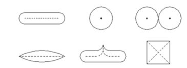
Fig. Region skeletons; small changes in border can have a significant effect on the skeleton.
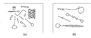
- Skeleton construction algorithms do not result in graphs but the transformation from skeletons to graphs is relatively straightforward.
- Consider first the medial axis skeleton, and assume that a minimum radius circle has been drawn from each point of the skeleton which has at least one point common with a region boundary.
- Let contact be each contiguous subset of the circle which is common to the circle and to the boundary.
- If a circle drawn from its center A has one contact only, A is a skeleton end-point.
- If point A has two contacts, it is a normal skeleton point.
- If A has three or more contacts, point A is a skeleton node-point.
Algorithm 6.9: Region graph construction from skeleton
1. Assign a point description to all skeleton points- end points, node-points, normal- points.
2. Let graph node- point be all end- points and node- points. Connect any two graph nodes by a graph edge if they are connected by a sequence of normal point in the region skeleton.
- It can be seen that boundary points of high curvature have the main influence on the graph.
- They are represented by graph nodes, and therefore influence the graph structure.
- If other than medial axis skeletons are used for graph construction, end-points can be defined as skeleton points having just one skeleton neighbor, normal-points as having two skeleton neighbors, and node-points as having at least three skeleton neighbors.
- It is no longer true that node-points are never neighbors and additional conditions must be used to decide when node-points should be represented as nodes in a graph and when they should not.
Region decomposition
- The decomposition approach is based on the idea that shape recognition is a hierarchical process.
- Shape primitives are defined at the lower level, primitives being the simplest elements that form the region.
- A graph is constructed at a higher level - nodes result from primitives, arcs describe the mutual primitive relations.
- Convex sets of pixels are one example of simple shape primitives.
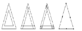
- The solution to the decomposition problem consists of two main steps:
- The first step is to segment a region into simpler subregions (primitives) and the second is the analysis of primitives.
- Primitives are simple enough to be successfully described using simple scalar shape properties.
- If subregions are represented by polygons, graph nodes bear the following information;
- Node type representing primary subregion or kernel.
- A number of vertices of the subregion represented by the node.
- Area of the subregion represented by the node.
- The main axis direction of the subregion is represented by the node.
- Center of gravity of the subregion represented by the node.
- If a graph is derived using attributes 1-4, the final description is translation invariant.
- A graph derived from attributes 1-3 is translation and rotation invariant.
- Derivation using the first two attributes results in a description that is size invariant in addition to possessing translation and rotation invariance.
Region neighborhood graphs
- Any time a region decomposition into subregions or an image decomposition into regions is available, the region or image can be represented by a region neighborhood graph (the region adjacency graph being a special case).
- This graph represents every region as a graph node, and nodes of neighboring regions are connected by edges.
- A region neighborhood graph can be constructed from a quadtree image representation, from run-length encoded image data, etc.
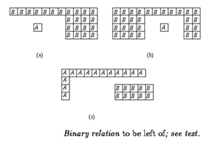
- Very often, the relative position of two regions can be used in the description process -- for example, a region A may be positioned to the left of a region B, or above B, or close to B, or a region C may lie between regions A and B, etc.
- We know the meaning of all of the given relations if A, B, C are points, but, with the exception of the relation to be close, they can become ambiguous if A, B, C are regions.
- For instance, human observers are generally satisfied with the definition:
- The center of gravity of A must be positioned to the left of the leftmost point of B and (logical AND) the rightmost pixel of A must be left of the rightmost pixel of B
Key takeaway
- A large group of shape description techniques is represented by heuristic approaches which yield acceptable results in a description of simple shapes.
- Heuristic region descriptors:
- Area,
- Rectangularity,
- Elongatedness,
- Direction,
- Compactness,
- Etc.
- These descriptors cannot be used for region reconstruction and do not work for more complex shapes.
Fig. Provides an overview of the approach that we propose for the analysis of 3D surfaces by persistence homology features. The input 3D surfaces are first projected to image-space to obtain depth maps as proposed in Zeppelzauer and Seidl. Next, depth maps are z-standardized and split into square patches. Patches are normalized and pre-filtered by Schmid or MR filters or CLBP. Next, topological descriptors are extracted as described in. Finally, feature selection is performed (optionally) before patch-wise classification to decrease the dimensionality of the feature vector and to reduce redundancies. The result is a class label for each surface patch, which were mapped back to the surface in Fig. For illustration.
Figure: Overview of the proposed approach.
Key takeaway
Fig. Provides an overview of the approach that we propose for the analysis of 3D surfaces by persistence homology features. The input 3D surfaces are first projected to image-space to obtain depth maps as proposed in Zeppelzauer and Seidl. Next, depth maps are z-standardized and split into square patches. Patches are normalized and pre-filtered by Schmid or MR filters or CLBP.
The pattern is everything around in this digital world. A pattern can either be seen physically or it can be observed mathematically by applying algorithms.
Example: The colors on the clothes, speech pattern, etc. In computer science, a pattern is represented using vector feature values.
What is Pattern Recognition?
Pattern recognition is the process of recognizing patterns by using a machine learning algorithm. Pattern recognition can be defined as the classification of data based on knowledge already gained or on statistical information extracted from patterns and/or their representation. One of the important aspects of pattern recognition is its application potential.
Examples: Speech recognition, speaker identification, multimedia document recognition (MDR), automatic medical diagnosis.
In a typical pattern recognition application, the raw data is processed and converted into a form that is amenable for a machine to use. Pattern recognition involves the classification and cluster of patterns.
- In classification, an appropriate class label is assigned to a pattern based on an abstraction that is generated using a set of training patterns or domain knowledge. Classification is used in supervised learning.
- Clustering generated a partition of the data which helps decision making, the specific decision-making activity of interest to us. Clustering is used in unsupervised learning.
Features may be represented as continuous, discrete, or discrete binary variables. A feature is a function of one or more measurements, computed so that it quantifies some significant characteristics of the object.
Example: consider our face then eyes, ears, nose, etc are features of the face.
A set of features that are taken together, forms the features vector.
Example: In the above example of a face, if all the features (eyes, ears, nose, etc) are taken together then the sequence is feature vector([eyes, ears, nose]). The feature vector is the sequence of features represented as a d-dimensional column vector. In the case of speech, MFCC (Mel-frequency Cepstral Coefficient) is the spectral features of the speech. The sequence of the first 13 features forms a feature vector.
Pattern recognition possesses the following features:
- Pattern recognition system should recognize a familiar pattern quickly and accurate
- Recognize and classify unfamiliar objects
- Accurately recognize shapes and objects from different angles
- Identify patterns and objects even when partly hidden
- Recognize patterns quickly with ease, and with automaticity.
Training and Learning in Pattern Recognition
Learning is a phenomenon through which a system gets trained and becomes adaptable to give results accurately. Learning is the most important phase as to how well the system performs on the data provided to the system depends on which algorithms are used on the data. The entire dataset is divided into two categories, one which is used in training the model i.e. Training set, and the other that is used in testing the model after training, i.e. Testing set.
- Training set:
The training set is used to build a model. It consists of a set of images that are used to train the system. Training rules and algorithms are used to give relevant information on how to associate input data with output decisions. The system is trained by applying these algorithms to the dataset, all the relevant information is extracted from the data, and results are obtained. Generally, 80% of the data of the dataset is taken for training data.
- Testing set:
Testing data is used to test the system. It is the set of data that is used to verify whether the system is producing the correct output after being trained or not. Generally, 20% of the data of the dataset is used for testing. Testing data is used to measure the accuracy of the system. For example, a system that identifies which category a particular flower belongs to can identify seven categories of flowers correctly out of ten and the rest others wrong, then the accuracy is 70 %
Real-time Examples and Explanations:
A pattern is a physical object or an abstract notion. While talking about the classes of animals, a description of an animal would be a pattern. While talking about various types of balls, then a description of a ball is a pattern. In the case balls considered as a pattern, the classes could be football, cricket ball, table tennis ball, etc. Given a new pattern, the class of the pattern is to be determined. The choice of attributes and representation of patterns is a very important step in pattern classification. A good representation is one that makes use of discriminating attributes and also reduces the computational burden in pattern classification.
An obvious representation of a pattern will be a vector. Each element of the vector can represent one attribute of the pattern. The first element of the vector will contain the value of the first attribute for the pattern being considered.
Example: While representing spherical objects, (25, 1) may be represented as a spherical object with 25 units of weight and 1 unit diameter. The class label can form a part of the vector. If spherical objects belong to class 1, the vector would be (25, 1, 1), where the first element represents the weight of the object, the second element, the diameter of the object and the third element represents the class of the object.
Advantages:
- Pattern recognition solves classification problems
- Pattern recognition solves the problem of fake biometric detection.
- It is useful for cloth pattern recognition for visually impaired blind people.
- It helps with speaker diarization.
- We can recognize a particular object from a different angle.
Disadvantages:
- The syntactic pattern recognition approach is complex to implement and it is a very slow process.
- Sometimes to get better accuracy, a larger dataset is required.
- It cannot explain why a particular object is recognized.
Example: my face vs my friend’s face.
Applications:
- Image processing, segmentation, and analysis
Pattern recognition is used to give human recognition intelligence to a machine which is required in image processing.
- Computer vision
Pattern recognition is used to extract meaningful features from given image/video samples and is used in computer vision for various applications like biological and biomedical imaging.
- Seismic analysis
The pattern recognition approach is used for the discovery, imaging, and interpretation of temporal patterns in seismic array recordings. Statistical pattern recognition is implemented and used in different types of seismic analysis models.
- Radar signal classification/analysis
Pattern recognition and signal processing methods are used in various applications of radar signal classifications like AP mine detection and identification.
- Speech recognition
The greatest success in speech recognition has been obtained using pattern recognition paradigms. It is used in various algorithms of speech recognition which tries to avoid the problems of using a phoneme level of description and treats larger units such as words as pattern
- Fingerprint identification
Fingerprint recognition technology is a dominant technology in the biometric market. A number of recognition methods have been used to perform fingerprint matching out of which pattern recognition approaches are widely used.
Key takeaway
The pattern is everything around in this digital world. A pattern can either be seen physically or it can be observed mathematically by applying algorithms.
Example: The colors on the clothes, speech pattern, etc. In computer science, a pattern is represented using vector feature values.
Pattern matching in computer vision refers to a set of computational techniques that enable the localization of a template pattern in a sample image or signal. Such a template pattern can be a specific facial feature, an object of known characteristics, or a speech pattern such as a word. Many of the challenges in computer vision, signal processing, and machine learning can be formulated and solved under the context of pattern matching terminology. An efficient solution to pattern search and matching should consist first in restricting search space to one in which the localization of the best match to a given pattern is not based on a direct comparison of a pixel by pixel values of the pattern and sample, but rather it is made on scale-invariant features. The use of these features, e.g. Harris corners or histogram-based matching, partially resolves the scale issue and reduces the matching problem to one for which only very few key points and their descriptors need to be aligned.
Many of our pattern recognition and machine learning algorithms are probabilistic in nature, employing statistical inference to find the best label for a given instance. For example, the use of deep learning techniques to localize and track objects in videos can also be formulated in the context of statistical pattern matching. After a learning phase, in which many examples of a desired target object’s features are learned to formulate a “pattern”, deep learning algorithms efficiently search and provide possible matches in any given test video. Another example can be behavior prediction of pedestrians in automatic driving assistance systems, based on learned trajectories of pedestrians.
In addition, multiple patterns can be searched simultaneously and be grouped into several categories or classes, for example, to determine whether a given email is “spam” or “non-spam” or to classify and grade agricultural products based on their characteristics and pathologies.
At RSIP Vision we develop and employ high-end pattern matching algorithms, tailor-made to the needs of our clients. Our custom pattern recognition and machine learning algorithms are used to achieve a wide variety of goals – from speech and facial recognition, through the automatic classification of white blood cells and dendritic cells, assistance in lens manufacturing, and up to monitoring animal behavior. We have a long experience in the development of in-house solutions and techniques to resolve challenges in computer vision, image processing, and machine learning. Please visit our project page to review RSIP Vision’s solutions in various industrial fields.
Key takeaway
Pattern matching in computer vision refers to a set of computational techniques that enable the localization of a template pattern in a sample image or signal. Such a template pattern can be a specific facial feature, an object of known characteristics, or a speech pattern such as a word. Many of the challenges in computer vision, signal processing, and machine learning can be formulated and solved under the context of pattern matching terminology.
References:
1. Rafael C. Gonzalez, Richard E. Woods, Digital Image Processing Pearson, Third Edition, 2010
2. Anil K. Jain, Fundamentals of Digital Image Processing Pearson, 2002.
3. Kenneth R. Castleman, Digital Image Processing Pearson, 2006.
4. Rafael C. Gonzalez, Richard E. Woods, Steven Eddins, Digital Image Processing using MATLAB Pearson Education, Inc., 2011.
5. D, E. Dudgeon, and RM. Mersereau, Multidimensional Digital Signal Processing Prentice Hall Professional Technical Reference, 1990.
6. William K. Pratt, Digital Image Processing John Wiley, New York, 2002
7. Milan Sonka et al Image processing, analysis and machine vision Brookes/Cole, Vikas Publishing House, 2nd edition, 1999