Unit - 2
Time domain and Frequency domain
The Impulse signal, Ramp signal, unit step and parabolic signals are used as the standard test signals. All these signals are explained below.
Impulse Signal:
This signal has zero amplitude everywhere except at the origin. Fig below shown the representation of Impulse signal.
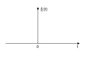
Fig 1 Unit Impulse Signal
The mathematical representations
A (t) = 0 for t ≠0
 dt = A e
Where A represent energy or area of the Laplace Transform of Impulse signal is
L [A (t)] = A
UNIT IMPULSE SIGNAL:
If A = 1
 (t) = 0 for t ≠0
L [ (t)] = 1
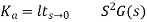
The transfer function of a linear time invariant
System is the Laplace transform of the impulse response of the system. If a unit impulse signal is applied to system then Laplace transform of the output c(s) is the transfer function G(s)
As we know G(s) = c(s)/R(S)
r(t) =  (t)
(t)
R(s) = L [ (t)] = 1
:. G(S) = C(s)
(b) Step signal:
Step signal of size A is a signal that change from zero level to A in zero time and stays there forever.
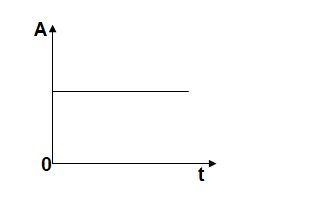
Fig 2 Unit Step Signal
r(t)= A t >=0
=0 t<0
L[r(t)] = R(s) = A/s
UNIT STEP SIGNAL: If the magnitude of the slip signal is I then it is called unit step signal.
u(t) = 1
t>=0
t<0
L[u(t)] = 1/s
(c) Ramp Signal:
The vamp signal increase linearly with time from initial value of zero at t= 0 as shown in fig is below
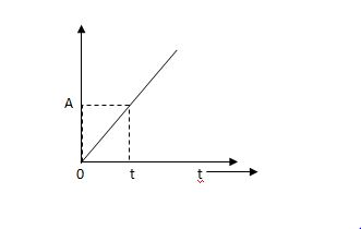
Fig 3 Ramp Signal
r(t) = At t>=0
=0 t<0
A is the slope of the line The Laplace transform of ramp signal is
L[r(t)] = R(s) = A/s2
(d) Parabolic Signal:
The instantaneous value of a parabolic signal varies as square of the time from an initial value of zero t=0. The signal representation in fig 14 below.

Fig 4 Parabolic Signal
r(t) At2 t>=0
=0 t<0
Then Laplace Transform is given as
R(s) = L[At2] = 2A/s3
If no error then E(t) =0, :. R(t) = c(t), output is tracking the input.
Steady state Errors signal (ess): - (t  )
)
Ess = t  e(t)
e(t)
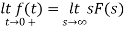
Using final values, the theorem
 = ess =
  S.E (s)
ess=  S[R(s)/1+G/(s)]
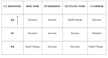
Key takeaway
If no error then E(t) =0, R(t) = c(t), output is tracking the input.
Steady state Errors signal (ess): - (t  )
)
ess = t  e(t)
e(t)
Using final values, the theorem
 = ess =
  S.E (s)
Examples
Q1) Find the initial value for the function f(t) = 2u(t)+3cost u(t)?
Sol:
f(t) = 2u(t)+3cost u(t)
F(s) = 
SF(s) = 2+ 
By initial value theorem
 = f(0+)
 =
=  2+
2+  = 5 = f(0+)
Hence, initial value of the function is 5
Q2) Find final value of the function F(s) = 
Sol:
F(s) = 
SF(s) = 
By final value theorem
 =
= 
 =
=  = 0.1
= 0.1
So, final value of the function is 0.1
Key takeaway
By initial value theorem
 = f(0+)
By final value theorem
 =
= 
Specifications:
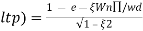
1) Rise Time (tp): The time taken by the output to reach the already status value for the first time is known as Rise time.
C(t) = 1-e- wnt/
wnt/ 1-
1- 2 sin (wdt+ø)
Sin (wd +ø) = 0
Wdt +ø = n
tr =n -ø/wd
-ø/wd
For first time so, n=1.
tr =  -ø/wd
-ø/wd
T=1/
2) Peak Time (tp)
The peak value attained by the output is called peak time. The time required by the output to reach this value is lp.
d(cct) /dt = 0 (maxima)
d(t)/dt = peak value
tp = n /wd for n=1
tp =  wd
wd
3) Peak Overshoot Value:
Maximum deviation of output from steady state value is called peak overshoot value (Mp).
(ltp) = 1 = Mp
(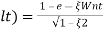 Sin(Wat + φ )
( Sin( Wd∏/Wd + φ)
Mp = e-∏ξ / √1 –ξ2
Condition 3 ξ = 1
C( S ) = R( S ) Wn2 / S2 + 2ξWnS + Wn2
C( S ) = Wn2 / S(S2 + 2WnS + Wn2) [ R(S) = 1/S ]
C( S ) = Wn2 / S( S2 + Wn2 )
C( t ) = 1 – e-Wnt + tWne-Wnt
The response is critically damped.
4) Settling Time (ts):
ts = 3 / ξWn (5%)
ts = 4 / ξWn (2%)
Key takeaway
Rise Time tr =  -ø/wd
-ø/wd
Peak Time tp = n /wd for n=1
tp =  wd
wd
Peak Overshoot Value
Mp% = e-∏ξ / √1 –ξ2
Settling Time
ts = 3 / ξWn (5%)
ts = 4 / ξWn (2%)
Examples
Q.1. The open loop transfer function of a system with unity feedback gain G(S) = 20 / S2 + 5S + 4. Determine the ξ, Mp, tr, tp.
Soln: Finding closed loop transfer function,
C(S) / R( S ) = G( S ) / 1 + G( S ) + H( S )
As it is unity feedback so, H(S) = 1
C(S)/R(S) = G(S)/1 + G(S)
= 20/S2 + 5S + 4/1 + 20/S2 + 5S + 4
C(S)/R(S) = 20/S2 + 5S + 24
Standard equation for second order system,
S2 + 2ξWnS + Wn2 = 0
We have,
S2 + 5S + 24 = 0
Wn2 = 24
Wn = 4.89 rad/sec
2ξWn = 5
(a). ξ = 5/2 x 4.89 = 0.511
(b). Mp% = e-∏ξ / √1 –ξ2 x 100
= e-∏ x 0.511 / √1 – (0.511)2 x 100
Mp% = 15.4%
(c). tr = ∏ - φ / Wd
φ = tan-1√1 – ξ2 / ξ
φ= tan-1√1 – (0.511)2 / (0.511)
φ = 1.03 rad.
tr = ∏ - 1.03/Wd
Wd = Wn√1 – ξ2
= 4.89 √1 – (0.511)2
Wd = 4.20 rad/sec
tr = ∏ - 1.03/4.20
tr = 502.34 msec
(d). tp = ∏/4.20 = 747.9 msec
Q.2. A second order system has Wn = 5 rad/sec and is ξ = 0.7 subjected to unit step input. Find (i) closed loop transfer function. (ii) Peak time (iii) Rise time (iv) Setteling time (v) Peak overshoot.
Soln: (i) The closed loop transfer function is
C(S)/R(S) = Wn2 / S2 + 2ξWnS + Wn2
= (5)2 / S2 + 2 x 0.7 x S + (5)2
C(S)/R(S) = 25 / S2 + 7s + 25
(ii). tp = ∏ / Wd
Wd = Wn√1 - ξ2
= 5√1 – (0.7)2
= 3.571 sec
(iii). tr = ∏ - φ/Wd
φ= tan-1√1 – ξ2 / ξ = 0.795 rad
tr = ∏ - 0.795 / 3.571
tr = 0.657 sec
(iv). For 2% settling time
ts = 4 / ξWn = 4 / 0.7 x 5
ts = 1.143 sec
(v). Mp = e-∏ξ / √1 –ξ2 x 100
Mp = 4.59%
Q.3. The open loop transfer function of a unity feedback control system is given by
G(S) = K/S(1 + ST)
Calculate the value by which k should be multiplied so that damping ratio is increased from 0.2 to 0.4?
Soln: C(S)/R(S) = G(S) / 1 + G(S)H(S) H(S) = 1
C(S)/R(S) = K/S(1 + ST) / 1 + K/S(1 + ST)
C(S)/R(S) = K/S(1 + ST) + K
C(S)/R(S) = K/T / S2 + S/T + K/T
For second order system,
S2 + 2ξWnS + Wn2
2ξWn = 1/T
ξ = 1/2WnT
Wn2 = K/T
Wn =√K/T
ξ = 1 / 2√K/T T
ξ = 1 / 2 √KT
Forξ1 = 0.2, for ξ2 = 0.4
ξ1 = 1 / 2 √K1T
ξ2 = 1 / 2 √K2T
ξ1/ ξ2 = √K2/K1
K2/K1 = (0.2/0.4)2
K2/K1 = 1 / 4
K1 = 4K2
Q.4. Consider the transfer function C(S)/R(S) = Wn2 / S2 + 2ξWnS + Wn2
Find ξ, Wn so that the system responds to a step input with 5% overshoot and settling time of 4 sec?
Soln:
Mp = 5% = 0.05
Mp = e-∏ξ / √1 –ξ2
0.05 = e-∏ξ / √1 –ξ2
Cn 0.05 = - ∏ξ / √1 –ξ2
-2.99 = - ∏ξ / √1 –ξ2
8.97(1 – ξ2) = ξ2∏2
0.91 – 0.91 ξ2 = ξ2
0.91 = 1.91 ξ2
ξ2 = 0.69
(ii). ts = 4/ ξWn
4 = 4/ ξWn
Wn = 1/ ξ = 1/ 0.69
Wn = 1.45 rad/sec
Transient Analysis of First Order System:
OLTF G(s) = 1/TS
CLTF c(s)/R(s) = 1/1+TS
CE: HTS = 0
S= -1/T
C(s) = R(s) [G(S)/1+G(s)]
C(s) = R(s)/1+TS
So, Calculating value of c(s), c(t) for different input
a) Unit Step:
R(t) = u(t)
R(s) = 1/s
C(s) = 1/s(1+ST)
1/s(1+ST) = A/s + o/1+TS
1/s(1+ST) = A/S + 0/1+TS
1= A(1+ST) + BS
AT +B =0
A = 1
B= -T
C(s) = 1/s + (-T)/1+TS
= 1+ (-T)/1-(-T) s = 1-I/n/1+ass+1/T =e-t/s
C(t) = [ 1-e-t/T]
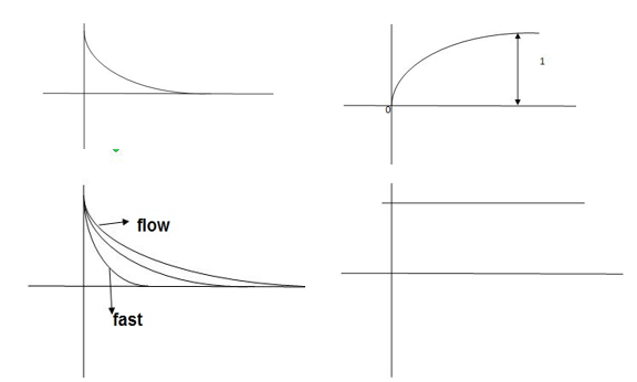
Fig 5 Output response for Unit Step input
Ramp:
R(t) = t
R(s) = 1/s2
C(s) = R(s) [G(s)/1+G(s)]
C(s) = 1/s2 1/(1+TS) + c
1/s2 (1+TS) = A/(s) + B/s2 + c(1+TS)
1 = A (s+s2. T) + B(1+TS) +cs2
TA +c = 0
A+TB =0
B =1
A = -T
C = T2
C(s) = -T/s + 1/s2 +T2/1+ST
=(-T) u(t) + t(u) + T e-t/T u(t)
= [ -T + t +Te-t/T u(t)
= [ -T+ t+Te-t/T] u(t)
C(s) = t- T+ Te-t/T
ess =  R(t) – c(t)
=  [ t- t+ 7-Te –t/T]
=  T( 1-e-t/T]
ess = The less the value of T the less in the errors.
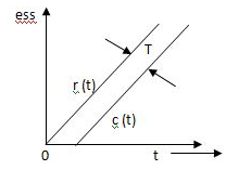
Fig 6 Output response for ramp input
From both the Cases input unit step, ramp Unit step
Unit Step Ramp
c(t) = 1-e-t/T r(t) = t
ess = e-t/T (r/t)-(t) c(t) = t- T+te-t/T
ess= e-t/T (r/t) (t) ess = T- Te-t/T
For :- for
 :-
:-
ess =0 ess = T
In both the vases (values of T) must be as small as possible (so, that e-t/T) must be as small as possible which gives us
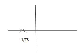
Fig 7 Location of poles
G(s) = 1/Ts
ATf = 1/1+TS
1st order system
Poles must be situated as far as possible from origin i.e., deeper and deeper into the left half of s-place. Thus, we get less errors.
Transient Analysis of Second Order System:
OLTF G(s) = k/s(1+TS)
CLTFC(s)/R(s) = k/k+s(1+Ts)
= k/s2+ s/T +k/T
Comparing above equation with standard 2nd order eqn
CLTF = wn2/s2+2rs wns+wn2
CEs2+2 wn s+wn2= 0
S= -2 wn±
wn±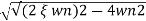 /2
/2
=2 wn±2wn
 /2
/2
S= wn±wn
wn±wn
S= - wn±wn
wn±wn
S= - wn ±wn
S= - wn ±gwn
Standard eqn:
T(s) = wn2/s2+2 wns+wn2
Our eqn T(s) = K/T/s2+1/T s+ K/T
Wn2 = k/T
2 wn = 1/T
2 k/T = 1/T
 k/T = 1/2T
 = 1/2T
  T/K
T/K
 = 1
= 1 2KT
2KT
Graphically showing the position of loops s1, s2 for offered of
As the characteristic Eqn. (location of poles) is dependent only on (wn constant for a given system)
S1 = - wn + jwn
  1-
1- 2
2
S2= - wn - jwn
 1-
1- 2
2
CASE 1: ( =0)
=0)
S1=jwn, S2, = -jwn
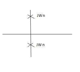
Fig 8 Location of poles for  =0
=0
Undamped
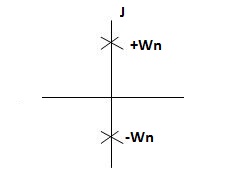
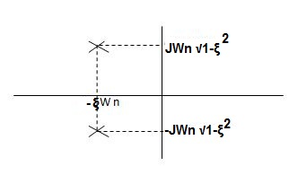
CASE 2:(0< <1)
<1)
S1= -wn + jwn  0.75
0.75
=-wn/2 +jwn (0.26)
S2 = -wn/2 – jwn (0.86)
Fig 9 Location of poles for  <1
<1
CASE:3 ( =1)
=1)
S1= S2 = - wn = -wn
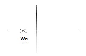
Fig 10 Location of poles for  =1
=1
CASE4: ( =-2)
=-2)
S1 = -2wn +jwn  -3
-3
=-2wn – jwn (1.73)
S1= -3.73wn
S2 = -2wn –jwn  -3
-3
= -2wn + jwn (1.73)
= -0.27  wn
wn
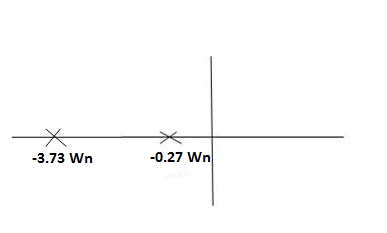
Fig 11 Location of poles for  >1
>1
Overdamped
Key takeaway
All practical systems are 2 order to, if R(e) =  (t) R(s) = 1. CLTF = 2nd order st eqn and hence already the system is possible.
CLTF = e(s)/ R(s) = wn2/s2+2 wns+wn2
Now calculating c(s), c(t) for different values of input
1) Impulse I/p
R(t) =  (t)
(t)
R(s) = 1
C(s) = R(s) wn2/s2+2 wns+wn2
C(s) = wn2/s2 +2 wn+wn2
Under this i/p (R(t) =  (t)) the output varies with different values of
  . So,
. So,
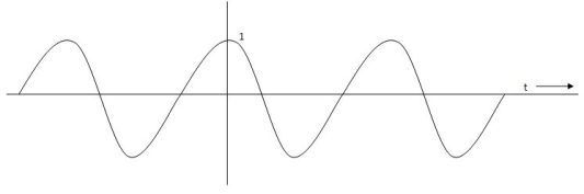
CONDITION 1: ( =0)
=0)
C(s) =wn2/s2 +wn2
Os2 +wn2 =0
S=+-jwn
C(t) = wn sinwnt
Sinwnt
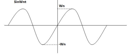
Fig 12 Undamped oscillations
As there in no damping i.e. oscillations at t= 0 are some at t  so, called UNDAMPED
CONDITION 2: 0<<1
c(s) = R(s) wn2/s22 wn+wn2 R(t) =
  (t)
(t)
R(s) =1
C(s) = wn2/s2+2 wns+wn2
CE
S2+2 wns +wn2 =0
S2, S1 = - wn ±jwn
  1-
1- 2
2
C(t) = e- wnt sin (wn
  )t
)t
Wd=wn )
)
C(t)=e- wnt sin (wdt)
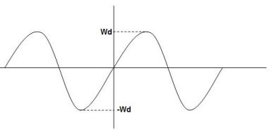
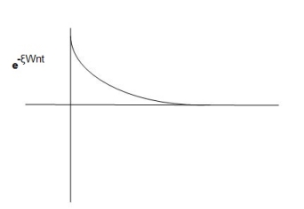
Fig 13 Underdamped oscillations
The oscillations are present but at t- infinity the Oscillations are 0 so, it is UNDERDAMPED
CONDITION 3:  =1
=1
C(s) = R(s) wn2/s2+2 wns+wn2
C(s)=wn2/S2 +2wns+wn2
=wn2/(s +wn)2
CE S= -Wn
Diagram
C(t)= w2n /(
 )2
)2
C(t)=
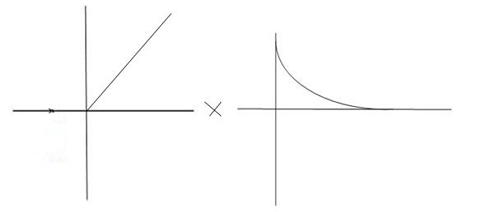
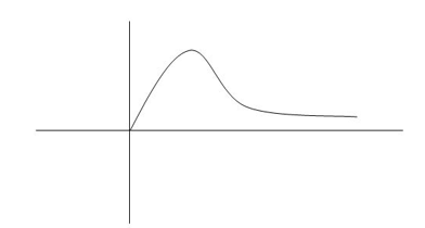
Fig 14 Critically damped oscillations
No damping obtained at  so is called CRITICALLY DAMPED.
CONDITIONS 4: >1
>1
C(s) = wn2/s22 wnS+Wn2
S1, s2 =  WN+-jwn
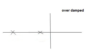
Fig 15 location of poles for over damped oscillations
b) UNIT Step Input:
R(s) = 1/s
C(s)/R(s) = wn2/s2+2 wns+wn2
C(s) = R(s) wn2 /s2 +2 wns+wn2
C(s) = R(s) wn2/s2+2 wns+wn2
C(s) = R(s) wn2/s2+2 wns+wn2
C(s) = wn2s(s2+2 wns+wn2)
C(t) = 1- e wnt/
wnt/ 1-es2 sin (wdt + ø)
Wd = wn 1-
1- 2
2
Ø= 
Where
Wd = Damping frequency of oscillations
Wn = natural frequency of oscillations
 wn = damping coefficient.
T= Time constant
Condition 1 = 0
= 0
C(s) = wn2 /s(s2+wn2)
C(t) = 1- e° sin wdt +ø
C(t)= 1- sin(wn +90)
C(t) = 1+cos wnt
Constant
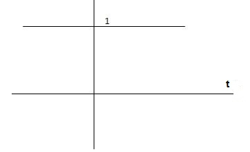
C(t) = 1+constant
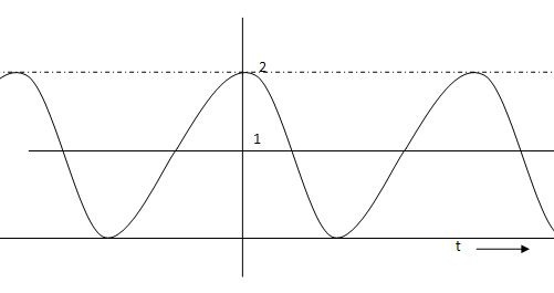
Fig 16 C(t) = 1+cos wnt
Condition 2: 0< <1
<1
C(s) =  /s2+
/s2+ wns +wn2
C(s) =1/s – s+ wn/s2+
 wns +wn2
=1/s – s+ wn/(s+
 wn)2+wd2-
  wn/(s+
 wn2) +wd2
Wd = wn  1-
1- 2
2
Taking Laplace inverse of above equation
L --1 s+ wn/(s+
 wn) +wd2= e-
 wnt cos wdt
L-1 s+ wn/(s+
 wn)2+wd2 = e-
 wnt sinWdt
C(t) = 1-e- wnt [coswdt +
 /
/ 1-
1- 2 sinwdt]
= 1-e wnt /
wnt / 1-
1- 2 sin [wdt +
  1-
1- 2/
2/ ] t>=0
C(t) = 1-e wnt/
wnt/ 1-
1- 2 sin(wdt+ø)
Ø =  1+
1+ 2/
2/
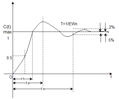
Fig 17 Transient Response of second order system
So, for difficult input, ess will be different Input still be
1. R(s) = unit step
2. R (s) = Ramp
3. R(s) = parabolic
1. R(s)= Unit step
R(t) = u(t)
R(s) = 1/s
Ess =  s[ R(s)/1+G(s)]
=  s[ys/1+G(s)]
ess=  1+1/1+G(s)
=1/1+lt G(s) s- 0
 (Position error coefficient)
Ess = 1/1+kp
2. R(s) = Ramp
R(t) = t
R(s) = 1/s2
ess=  s[ R(s)/1+G(s)]
=  s[ys2/1+G(s)]
=  1/s(1+G(S)
= 1/s+SG(s)
ess= l/s-0 SG (s)
ess =  t L/SG (s)
 (velocity errors coefficient)
ess = L/Kv
3. Parabolic
R(t) = t2
R(s) =1/s3
Ess =  s[ R(s)/1+G(s)]
=  s(1/s3)/1+G(s)
=  1/s2+s2G(s)
Ess =  1/s2G(s)
Acceleration error coefficient
ess = 1/ka
Input Error coefficient
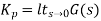
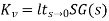
(1) Unit step ess= 1/1+kv kv =  G(S)
G(S)
(2) Ramp ess= 1/kv kv =  sG(s)
sG(s)
(3) Parabolic ess= 1/ka ka =  s2 G(s)
Now finding errors in type 0,1,2 system
1) Type 0:
G(s) = 1/(s+a) (s+b)
Kp:
Kp =
= 1/(s+a)(s+b)
Kp= 1/ab
Ess=1/1+np = 1/1+(1/ab) 
o/p not locking the input
Kv:
Kv =  s G(s)
=  s/(s+a) (s+b)
= s/(s+a) (s+b)
Kv = 0
ess = 1/kv = 
o/p not locating the input
Ka:
Ka =  s2 G(s)
=  s2 /(s+a) (s+b)
Ka =0
ess = 1/ka = 
o/p not locking the input
2) Type –I:
G(s) = 1/s(s+a) (s+b)
Kp:
Kp =  G(s)
G(s)
= 1/s(s2+as+ab)
Kp = 1/0 = 
ess = 1/1+kp = 0
o/p is tracking the input
Kv:
Kv =  S G(s)
= 1/(s+a) (s+b)
=1/ab
Kv = 1/ab
ess =1/ka = ab 
o/p is not tracking the input
Ka:
Ka=  s2G(s)
=  s2 /s(s+a)(s+b)
=  s/(s+a)(s+b)
Ka= 0
Ess = 1/ka = 
O/p is not tracking the input
3) Type 2:
G(s) = 1+/(s2(s+a) (s+b)
Kp:
Kp =  G(s)
G(s)
=  1/s2 (s+a) (s+b)
Kp = 
ess = 1/1+kp = 0
o/p tracking the i/p
Kv:
Kv = s G(s)
= 1/s(s+a) (1+b)
kv = 
ess =1/ = 0
= 0
o/p tracking the o/p
Ka:
Ka=  s2G(s)
= 1/(s+a) (s+b)
Ka = 1/ab
ess = 1/(yab) ≠0
o/p not locking the i/p
Key takeaway:
ess Type 0 Type 1 Type 2 |
Unit step ≠0 0 0 |
Ramp  |
Parabolic  |
The dynamic error constant coefficient method is a generalized method to include inputs of any arbitrary function of time. For a unity feedback system,
E(s)/R(s) = 1/1+G(s) =F(s)
The function F(s) can also be written as
E(s)/R(s) = 1/1+G(s) = C0+C1s+C2s2+C3s3+…..
C0 C1 C2 C3 are defined as dynamic error coefficients
E(s) = C0R(s)+ C1 sR(s)+ C2/2! s2R(s) …..
The generalised error coefficients are calculated as follows


Correlation between static and dynamic error constants


The feedback systems are having many advantages over the non-feedback system as we have seen earlier. So, some performance parameters can be controlled through this feedback system such as sensitivity, noise etc. Sensitivity is a parameter which forecasts the effectiveness of feedback in reducing the influence of these variations on system performance.
The output of the open loop system is given by
C(s) = G(s)R(s)
Now due to variation in parameters G(s) changes to [G(s)+ G(s)]. The output will now become
C(s)+ C(s) = [G(s)+
 G(s)] R(s)
 C(s) =
  G(s)R(s)
For closed loop system the output is given as
C(s) =  R(s)
R(s)
Now due to variation in parameters it becomes
C(s)+ C(s) =
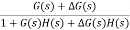 R(s)
R(s)
The above equation shows that if there is variation in parameters then G(s) is reduced by factor of 1+G(s)H(s). The variation in overall transfer function T(s) due to change in G(s) is defined as sensitivity.
Sensitivity = 
When there is small change in G(s) then sensitivity becomes

 : Sensitivity of T w.r.t G
For closed loop system the sensitivity will be
 =
=  x
x  =
= 
For open loop system
 = 1
= 1
As T=G
The sensitivity of T w.r.t H is given as
 =G [
=G [ ]
]  =
= 
The above equation shows that for large values of GH sensitivity of the feedback system w.r.t H approaches to unity.
Key takeaway
For closed loop system the sensitivity w.r.t G is reduced by a factor of (1+GH) as compared to the open loop system.
Effects of controller are viewed on time response and stability.
Fig 18 Controller with unity feedback system
Gc(S) = TF of the controller
G(S) = OLTF without controller
G’(S) = Gc(S).G(S)
= OLTF with controller
1. Proportional (P) Controller –
Proportional means scalar Multiplier.
Gc(S) = Kp Stability can be controlled
Q. G(S) = 1/S(S + 8)
CLTF = 1/S2 + 8S + 1
w2n = 1
wn = 1
2ξWn = 8
ξ = 4
ξ>/1 so, overdamped.
Now introducing Gc(S) = K
G’(S) = Kp/S(S + 8)
CLTF = Kp/S2 + 8S + Kp
wn = √Kp
2 ξwn = 8
ξ = 4/√Kp
If,
Kp = 16; ξ = 1; critically damped
Kp> 16; ξ< 1; undamped
Kp< 16; ξ> 1; overdamped
2. Integral (I) controller –
The transfer function of this controller is
Gc(S) = Ki/S
Integral controller is used to improve the steady state response or reduce the steady state error.
Fig 19 Integral Controller
G’(S) = Gc(S).G(S)
G(S) = 1/S + 5, Gc(S) = Ki/S
G’(S) = Ki/S(S + 5). After applying the Gc(S) the type of system is increasing and hence, the steady state error is decreasing (Refer Time Response).
Disadvantage -
By using integral controller, the stability of closed loop system decreases.
G(S) = 1/S + 5
Fig 20 Pole Locations For given system
G’(S) = Ki/S(S + 5)
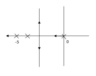
Fig 21 Pole Location after Integral controller
Fig(20), is more stable than (21) as more the away the pole from origin (imaginary axis) more is the stability.
Q. G(S) = 1/(S + 5)(S + 10)
G’(S) = Kp/S(S + 5)(S + 10)
G(S) = 1/(S + 5)(S + 10)
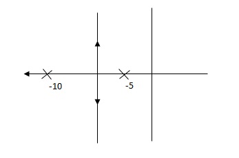
Fig 22 Root Locus Without controller
G’(S) = Ki/S(S + 5)(S + 10)
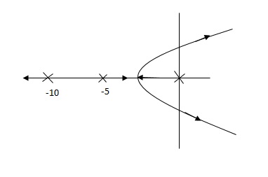
Fig 23 Root Locus Without controller
So, Fig 23 is less stable at root locus lies on the R.H.S
3. Derivative (D) Controller -
Gc(S) = Kd(S)
They are used to improve the stability.

Fig 24 Derivative controller system
G’(S) = KdS/S2(S + 10)
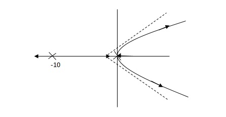
Fig 25 Root Locus for system without controller
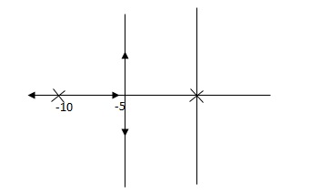
Fig 26 Root locus with controller
Fig 26 is stable i.e. more stable than the Fig 25.
Disadvantage –
It increases the steady state i.e. o/p will not track the input at steady state.
4. Proportional Plus Integral [PI] controller -
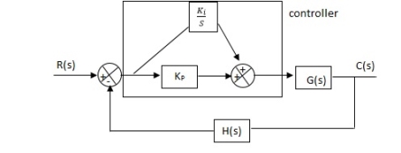
Fig 27 PI controller
Gc(S) = KpS + Ki/S
The steady state error will decrease and the stability will depend on Kp i.e. if Kp is increased/decreased than according to it stability will change (Kpα stability).
Used to reduce ess without much affecting the stability.
5. Proportional Plus Derivative (PD) Controller -
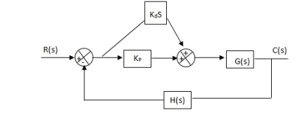
Fig 28 PD controller
Used to improve the stability without affecting much the steady state error.
6. PID controller -
Gc(S) = Kp + Ki/S + KdS
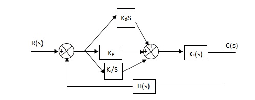
Fig 29 PID Controller
It improves the stability. It decreases the steady state error and both are proportional to Kp.
Key takeaway
Example-1 The block diagram of a system using PI controllers is shown in the figure below Calculate:
(a). The steady state without and with controller for unit step input?
(b). Determine TF of newly constructed sys. With controller so, that a CL Poles is located at -5?
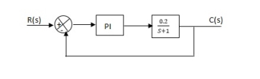
Fig 30 Block diagram with PI controller
(a). Without:
C(S)/R(S) = 0.2/(S + 1)
C(S) = R(S) 0.2/(S + 1) + 0.2
For unit step
Ess = 1/1 + Kp
Kp = lt G(S)
S 0
= lt 0.2/(S + 1)
S 0
Kp = 0.2
Ess = 1/1.2 = 5/6 = 0.8
(b). With controller:
Gc(S) = Kp + Ki/S
G’(S) = Gc(S).G(S)
= ( Kp + Ki/S )0.2/(S + 1)
= (KpS + Ki)0.2/S(S + 1)
Ess = 1/1 + Kp = 0
So, the value of ess is decreased.
(b). Given
Kpi/Kp = 0.1
G’(S) = (Kp + Ki/S)(0.2/S + 1)
= (KpS + Ki)0.2/S(S + 1)
As a pole is to be added so, we have to examine the CE,
1 + G’(S) = 0
1 + (Kp + Ki)0.2/S(S + 1) = 0
S2 + S + 0.2KpS + 0.2Ki = 0
S2 + (0.2Kp + 1)S + 0.2Ki = 0
Given,
Kpi = 0.1Ki
Kp = 10Ki
S2 + (2Ki + 1)S + 0.2Ki = 0
Pole at S = -5
25 + (2Ki + 1)(-5) + 0.2Ki = 0
-10Ki – 5 + 25 + 0.2Ki = 0
-9.8Ki = -20
Ki = 2.05
Kp = 10Ki
= 20.5
Now,
G’(S) = (KpS + Ki)(0.2)/S(S + 1)
= (20.5S + 2.05)(0.2)/S(S + 1)
G’(S) = 4.1S + 0.41/S(S + 1)
Example-2 The block diagram of a system using Pd controller is shown, the PD is used to increase ξ to 0.8. Determine the T.F of controller?
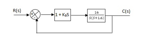
Fig 31 Block diagram with PD controller
(1). Kp = 1
Without controller:
C(S)/R(S) = 16/S2 + 1.6S + 16
wn = 4
2 ξwn = 16
ξ = 1.6/2 x 4 = 0.2
(b). With derivative:
ξS = 0.2 to 0.8
Undamped to critically damped,
G’(S) = (1 + KdS)(16)/(S2 + 1.6S)
CE:
S2 + 1.6S + 16(1 + KdS) = 0
S2 + (1.6 + Kd)S + 16 = 0
2 ξwn = 1.6 + Kd1.6
wn = 4
ξS = 0.8
2 x 4 x 0.8 = 1.6 + Kd1.6
6.4 – 1.6 = Kd1.6
4.8/16 = Kd
Kd = 0.3
TF = (1 + 0.3S)16/S(S + 16)
References:
1. I. J. Nagrath and M. Gopal, “Control Systems Engineering”, New Age International, 2009.
2. K. Ogata, “Modern Control Engineering”, Prentice Hall, 1991
3. M. Gopal, “Control Systems: Principles and Design”, McGraw Hill Education, 1997.
4. B. C. Kuo, “Automatic Control System”, Prentice Hall, 1995.


