Unit - 3
Stability Criterion
Routh Hurwitz stability criterion
It states that the system is stable if and only if all the elements is the first column have the same algebraic sign. If all elements are not of the same sign then the number of sign changes of elements in first column equals the number of roots of the characteristic equation in the right half of S-plane.
Consider the following characteristic equation:
a0 Sn + a1 Sn-1 ………….an = 0 where a0,a1,,,,,,,,,,,,,,,,,,,,an have same sign and are non-zero.
Step1 Arrange coefficients in rows
Row1 ao a2 a4
Row2 a1 a3 a5
Step2 Find third row from above two rows
Row1 a0 a2 a4
Row2 a1 a3 a5
Row3 a1 a3 a5
a1 = 
 =
= 
a3 = 
 =
= 
Continue the same procedure to find new rows.
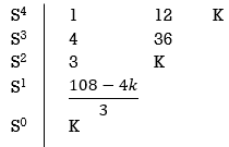
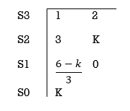
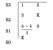
Q1) for the given polynomials below determine the stability of the system
S4+2S3+3S2+4S+5=0
Sol:
Arranging Coefficient in Rows.
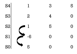
For row S2 first term
S2 =  = 1
= 1
For row S2 Second term
S2 =  = 5
= 5
For row S1:
S1 =  = -6
= -6
For row S0
S0 =  = 5
= 5
As there are two sign change in the first column, So there are two roots or right half of S-plane making system unstable.
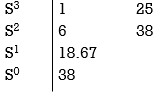
Q2. Using Routh criterion determine the stability of the system with characteristic equation S4+8S3+18S2+16S+S = 0
Sol: Arrange in rows.

For row S2 first element
S1 =  = 16
= 16
Second terms =  = 5
= 5
For S1
First element =  = 13.5
For S0
First element = 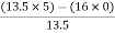 = 5
= 5
As there is no sign change for first column so all roots are is left half of S-plane and hence system is stable.
Special Cases of Routh Hurwitz Criterions
(I) When first element of any row is zero.
In this case the zero is replaced by a very small positive number E and rest of the array is evaluated.
Eg.(1) Consider the following equation
S3+S+2 = 0
Replacing 0 by E
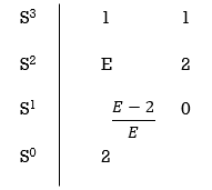
Now when E  0, values in column 1 becomes
Two sign changes hence two roots on right side of S-plans
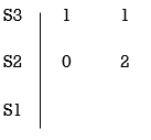
(II) When any one row is having all its terms zero.
When array one row of Routh Hurwitz table is zero, it shown that the X is attests one pair of roots which lies radially opposite to each other in this case the array can be completed by auxiliary polynomial. It is the polynomial row first above row zero.
Consider following example
S3 + 5S2 + 6S + 30
For forming auxiliary equation, selecting row first above row hang all terms zero.
A(s) = 5S2 e 30
 = 10s e0.
Again forming Routh array

No sign change in column one the roots of Auxiliary equation A(s)=5s2+ 30-0
5s2+30 = 0
S2 α 6= 0
S = ± j 
Both lie on imaginary axis so system is marginally stable.
Q3. Determine the stability of the system represent by following characteristic equations using Routh criterion
1) S4 + 3s3 + 8s2 + 4s +3 = 0
2) S4 + 9s3 + 4S2 – 36s -32 = 0
1) S4+3s3+8s2+4s+3=0
No sign change in first column to no rows on right half of S-plane system stable.
2) S4 + 9s3 + 4S2 – 36s -32 = 0
Special case II of Routh Hurwitz criterion forming auxiliary equation
A1 (s) = 8S2 – 32 = 0
 = 16S – 0 =0
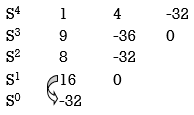
One sign change so, one root lies on right half S-plane hence system is unstable.
Q4. For using feedback open loop transfer function G(s) = 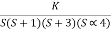
Find range of k for stability
Soln: Findlay characteristics equation.
CE = 1+G (s) H(s) = 0
H(s) =1 using feedback
CE = 1+ G(s)
1+ 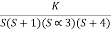 = 0
= 0
S(S+1)(S+3)(S+4)+k = 0
(S2+5)(S2+7Sα12)αK = 0
S4α7S3α1252+S3α7S2α125αK = 0
S4+8S3α19S2+125+k = 0
By Routh Hurwitz Criterion
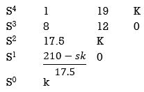
For system to be stable the range of K is 0< K <  .
.
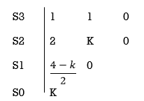
Q5. The characteristic equation for certain feedback control system is given S4 +4S3+ 12S2+36S+K. Find range of K for system to be stable.
Sol:
S4+4S3α12S2+36SαK = 0
For stability K>0
 > 0
> 0
K < 27
Range of K will be 0 < K < 27
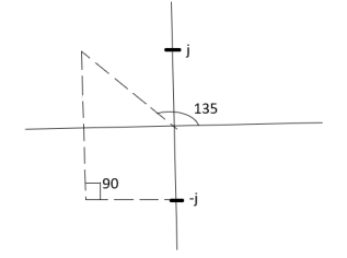
Relative Stability:
Routh stability criterion deals about absolute stability of any closed loop system. For relative stability we need to shift the S-plane and the apply the Routh criterion.

Fig. Location of Pole for relative stability
The above fig 10 shows the characteristic equation is modified by shifting the origin of S-plane to S1= - .
.
S = Z-S1
After substituting new valve of S =(Z-S1) applying Routh stability criterion, the number of sign changes in first column is the number of roots on right half of S-plane
Q6. Check if all roots of equation
S3+6S2+25S+38 = 0, have real poll more negative than -1.
Soln:
No sign change in first column, hence all roots are in left half of S-plane.
Replacing S = Z-1. In above equation
(Z-1)3+6(Z-1)2+25(Z-1)+38 = 0
Z3+ Z23+16Z+18=0
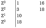
No sign change in first column roots lie on left half of Z-plane hence all roots of original equation in S-domain lie to left half 0f S = -1
Key takeaway
Special Cases of Routh Hurwitz Criterions
(I) When first element of any row is zero.
In this case the zero is replaced by a very small positive number E and rest of the array is evaluated.
(II) When any one row is having all its terms zero.
When array one row of Routh Hurwitz table is zero, it shown that the X is attests one pair of roots which lies radially opposite to each other in this case the array can be completed by auxiliary polynomial. It is the polynomial row first above row zero.
Introduction
The root locus is graphical produce for determining the stability of a control system which is determined by the location of the poles. The poles are nothing but the roots of the characteristic equation.
Properties of Root Locus
- It is symmetrical to the real axis.
- The number of branches of the root locus is equal to the number of maxes. (poles or zero).
- Starting point (k=0) Endpoint(k—>∞)
(open-loop poles) (open loop zeros)
4. A point on the real axis lies on the root locus if many open-loop poles or zero to the right side of that point is odd in number.
5. Value of K anywhere on the root locus is given as
K = 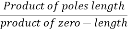
6. I)If poles > zeros then (Þ-z) branches will terminate at ∞ (where k=∞)
II)If Z > P, then (Z-P) branches will start from ∞ (K = 0)
7. When P>Z, (P-Z) branches will terminate at ∞ (open loop zeros). But by which path. So the path is shown by asymptotes and this asymptote is given by
Asymptote =  q = o,1,2……(P-Z-1)
8. These asymptotes intersect the real axis at a single point and this point is known as centroid.
Centroid = 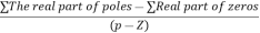
9. Breakaway and break-in point when the root locus lies between two poles it's called break-in point.
Centroid and Breakaway points are not the same
Differentials the characteristic equation and equate to zero 
10. The angle of arrival and angle of departure this print is used when the roots are complex.
The angle of departure - for complex poles
The angle of arrival – for complex zero.
11. The intersection of root locus with an imaginary axis can be calculated by Routh Hurwitz. By calculating the value of k at intersection point (we can comment about system stability) so by knowing the values of k at intersection point (imaginary axis) the valve of s at that point can also be calculated.
Stable: If the root low (all the branches) lies within the left side of the S-plane.
Conditionally Stable: If some part of the root locus lies on the left half and the same
The part on the right of the S-plane then is conditionally stable.
Unstable: If the root locus lies completely on the right side of the S-plane then it is unstable.
The values of S which satisfy both the angle and magnitude conditions are the roots of the characteristic equation.
Angle condition:
LG(S)H(S) = +-1800(2 KH) (K = 1,2,3,--)
If the angle is an odd multiple of 1800 it satisfies the above condition.
Magnitude condition:
| G(S)H(S) = 1 | at any point on the root locus. The magnitude condition can be applied only if the angle condition is satisfied.
Design aspects of Root Locus
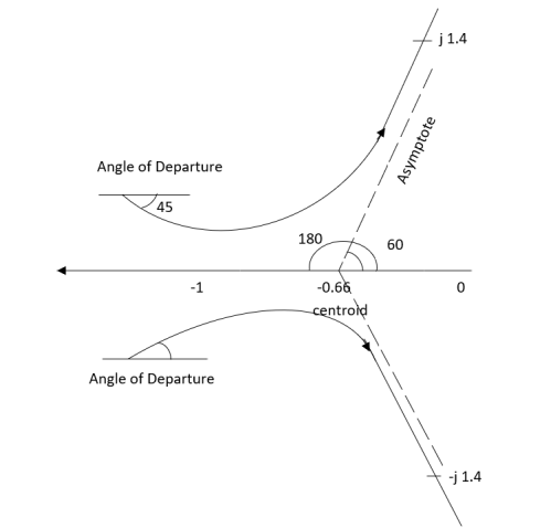
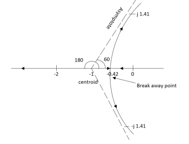
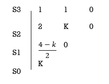
Q1. Sketch the root locus for given open-loop transfer function G(S) =  .
.
Soln: 1) G(s) = 
Number of Zeros = 0
Number of polls S = (0, -1+j, -1-j) = (3).
1) Number of Branches = max (P, Z) = max (3, 0) = 3.
2) As there are no zeros in the system so, all branches terminate at infinity.
3) As P>Z, branches terminate at infinity through the path shown by asymptotes
Asymptote =  × 180° q = 0, 1, 2………..(p-z-1)
P=3, Z=0.
q= 0, 1, 2.
For q=0
Asymptote = 1/3 × 180° = 60°
For q=1
Asymptote =  × 180°
= 180°
For q=2
Asymptote =  × 180° = 300°
Asymptotes = 60°,180°,300°.
4) Asymptote intersects the real axis at the centroid
Centroid =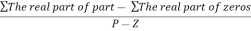
= 
Centroid = -0.66
5) As poles are complex so the angle of departure
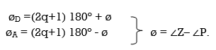
øD = (2q+1)×180°+ø
ø = ∠Z –∠P.
Calculating ø for S=0
Join all the other poles with S=0
ø = ∠Z –∠P.
= 0-(315°+45°)
= -360°
ØD = (2q + 1)180 + ø.
= 180° - 360°
ØD = -180° (for q=0)
= 180° (for q=1)
=540° (for q=2)
Calculation ØD for pole at (-1+j)

ø = ∠Z –∠P.
= 0 –(135°+90°)
= -225°
ØD = (2q+1) 180°+ø.
= 180-225°
= -45°
ØD = -45° (for q = 0)
= 315° (for q = 1)
= 675° (for q =2)
6) The crossing point on the imaginary axis can be calculated by Routh Hurwitz the characteristic equation is.
1+G(s) H (s) = 0
1+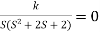
S (S2+2s+2)+k = 0
S3+2s2+2s+K = 0
For stability  > 0. And K > 0.
0<K<2.
So, when K=2 root locus crosses imaginary axis
S3 + 2S2 + 2S + 2 =0
For k
Sn-1 = 0 n : no. Of intersection
S2-1 = 0 at imaginary axis
S1 = 0
 = 0
= 0
K<4
For Sn = 0 for valve of S at that K
S2 = 0
2S2 + K = 0
2S2 + 2 = 0
2(S2 +1) = 0
32 = -2
S = ± j 
The root locus plot is shown in figure.
Q2. Sketch the root locus plot for the following open-loop transfer function
G(s) = 
- Number of zero = 0, number of poles = 3
2. As P>Z, branches will terminate at infinity
3. There are no zeros so all branches will terminate at infinity.
4. The path for the branches is shown by asymptote
Asymptote =  ×180°. q=0,1,………p-z-1
P=3, Z=0
q= 0,1,2.
For q = 0
Asymptote =  × 180° = 60.
For q=1
Asymptote =  × 180° = 180°
For q=2
Asymptote =  × 180° = 300°
5. Asymptote intersects the real axis at the centroid
Centroid = 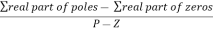
=  = -1
= -1
6. As root locus lies between poles S= 0, and S= -1
So, calculating the breakaway point.
 = 0
= 0
The characteristic equation is
1+ G(s) H (s) = 0.
1+  = 0
= 0
K = -(S3+3S2+2s)
 = 3S2+6s+2 = 0
3s2+6s+2 = 0
S = -0.423, -1.577.
So, the breakaway point is at S=-0.423
Because root locus is between S= 0 and S= -1
7. The intersection of the root locus with the imaginary axis is given by the Routh criterion.
Characteristics equation is
S3+3S3+2s+K = 0
For k
Sn-1= 0 n: no. Of intersection with imaginary axis
n=2
S1 = 0
 = 0
= 0
K < 6 Valve of S at the above valve of K
Sn = 0
S2 = 0
3S2 + K =0
3S2 +6 = 0
S2 + 2 = 0
S = ±  j
j
The root locus plot is shown in fig.

Q3. Plot the root locus for the given open-loop transfer function
G(s) = 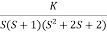
- Number of zeros = 0 number of poles = 4
P = (S=0,-1,-1+j,-1-j) = 4
2. As P>Z all the branches will terminated at infinity.
3. As no zeros so all branches terminate at infinity.
4. The path for branches is shown by asymptote.
Asymptote =  q = 0,1,…..(Þ-z-1)
q=0,1,2,3. (P-Z = 4-0)
For q=0
Asymptote =  ×180° =45°
For q=1
Asymptote =  ×180° =135°
For q=2
Asymptote =  ×180° =225°
For q=3
Asymptote =  ×180° =315°
5. Asymptote intersects real axis at unmarried
Centroid = 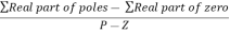
Centroid =  =
=  = -0.75
6) As poles are complex so angle of departure is
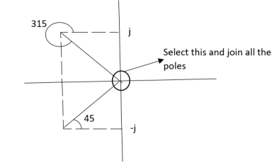
ØD = (2q+1) ×180 + ø ø = ∠Z –∠P.
Calculating Ø for S=0
ø = ∠Z –∠P.
= 0 –[315° + 45°]
Ø = -360°
For q = 0
ØD = (2q+1) 180° + Ø
= 180 - 360°
ØD = -180°
b) Calculating Ø for S=-1+j
ø = ∠Z –∠P.
= 0-[135° + 90° + 90°]
Ø = -315°
For q=0
ØD= (2q+1) 180° +Ø
= 180° -315°
ØD = -135°
ØD for S=1+j will be ØD = 45°
7) As the root locus lie between S=0 and S=-1
So, the breakaway point is calculated

1+ G(s)H(s) = 0
1+ 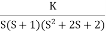 = 0
= 0
(S2+S)(S2 +2S+2) + K =0
K = -[S4+S3+2s3+2s2+2s2+2s]
 = 4S3+9S2+8S+2=0
S = -0.39, -0.93, -0.93.
The breakaway point is at S = -0.39 as root locus exists between S= 0 and S=-1
8) Intersection of root locus with imaginary axis is given by Routh Hurwitz
I + G(s) H(s) = 0
K+S4+3S3+4S2+2S=0
For system to be stable
 >0
>0
6.66>3K
0<K<2.22.
For K = 2.22
3.3352+K =0
3.3352 + 2.22 = 0
S2 = -0.66
S = ± j 0.816.
The root locus plot is shown in figure.

Q4. Plot the root locus for the open-loop system
G(s) = 
1) Number of zero = 0 number of poles = 4 located at S=0, -2, -1+j, -1-j.
2) As no zeros are present so all branches terminated at infinity.
3) As P>Z, the path for branches is shown by asymptote
Asymptote = 
q = 0,1,2……p-z-1
For q = 0
Asymptote = 45°
q=1
Asymptote = 135°
q=2
Asymptote = 225°
q=3
Asymptote = 315°
4) Asymptote intersects real axis at centroid.
Centroid = 
= 
Centroid = -1.
5) As poles are complex so angle of departure is
ØD=(2q+1)180° + Ø
ø = ∠Z –∠P
= 0-[135°+45°+90°]
= 180°- 270°
ØD = -90°
6) As root locus lies between two poles so calculating point. The characteristic equation is
1+ G(s)H(s) = 0
1+ = 0.
= 0.
K = -[S4+2S3+2S2+2S3+4S2+4S]
K = -[S4+4S3+6S2+4S]
 = 0
= 0
 = 4s3+12s2+12s+4=0
S = -1
So, breakaway point is at S = -1
7) Intersection of root locus with imaginary axis is given by Routh Hurwitz.
S4+4S3+6S2+4s+K = 0

 ≤ 0
≤ 0
K≤5.
For K=5 valve of S will be.
5S2+K = 0
5S2+5 = 0
S2 +1 = 0
S2 = -1
S = ±j.
The root locus is shown in figure.

Q5. Plot the root locus for the open-loop transfer function G(s) = 
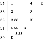
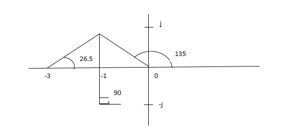
- Number of zeros = 0. Number of poles = 4 located at S=0, -3, -1+j, -1-j.
2. As no. Zero so all branches terminate at infinity.
3. The asymptote shows the both to the branches terminating at infinity.
Asymptote =  q=0,1,….(p-z).
For q = 0
Asymptote = 45
For q = 1
Asymptote = 135
For q = 2
Asymptote = 225
For q = 3
Asymptote = 315
(4). The asymptote intersects real axis at centroid.
Centroid = ∑Real part of poles - ∑Real part of zero / P – Z
= [-3-1-1] – 0 / 4 – 0
Centroid = -1.25
(5). As poles are complex so angle of departure
φD = (29 + 1)180 + φ

ø = ∠Z –∠P.
= 0 – [ 135 + 26.5 + 90 ]
= -251.56
For q = 0
φD = (29 + 1)180 + φ
= 180 – 215.5
φD = - 71.56
(6). Break away point dk / ds = 0 is at S = -2.28.
(7). The intersection of root locus on imaginary axis is given by Routh Hurwitz.
1 + G(S)H(S) = 0
K + S4 + 3S3 + 2S3 + 6S2 + 2S2 + 6S = 0
S4 1 8 K
S3 5 6
S2 34/5 K
S1 40.8 – 5K/6.8
K ≤ 8.16
For K = 8.16 value of S will be
6.8 S2 + K = 0
6.8 S2 + 8.16 = 0
S2 = - 1.2
S = ± j1.09
The plot is shown in figure.
Q.6. Sketch the root locus for open loop transfer function.
G(S) = K(S + 6)/S(S + 4)
- Number of zeros = 1(S = -6)
Number of poles = 2(S = 0, -4)
2. As P > Z one branch will terminate at infinity and the other at S = -6.
3. For Break away and breaking point
1 + G(S)H(S) = 0
1 + K(S + 6)/S(S + 4) = 0
Dk/ds = 0
S2 + 12S + 24 = 0
S = -9.5, -2.5
Breakaway point is at -2.5 and Break in point is at -9.5.
4. Root locus will be in the form of a circle. So finding the centre and radius. Let S = + jw.
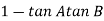
G( + jw) = K( + jw + 6)/( + jw)( + jw + 4 ) = +- π
Tan-1 w/ + 6 - tan-1 w/ – tan-1 w / + 4 = - π
Taking tan of both sides.
w/ + w/ + 4 / 1 – w/ w/ + 4 = tan π + w / + 6 / 1 - tan π w/ + 6
w/ + w/ + 4 = w/ + 6[ 1 – w2 / ( + 4) ]
(2 + 4)( + 6) = (2 + 4 – w2)
2 2 + 12 + 4 + 24 = 2 + 4 – w2
22 + 12 + 24 = 2 – w2
2 + 12 – w2 + 24 = 0
Adding 36 on both sides
( + 6)2 + (w + 0)2 = 12
The above equation shows circle with radius 3.46 and center(-6, 0) the plot is shown in figure.

Construction of Root-loci
Q1. Sketch the root locus for given open loop transfer function G(S) =  .
.
Soln:
1) G(s) = 
Number of Zeros = 0
Number of polls S = (0, -1+j, -1-j) = (3).
1) Number of Branches = max (P, Z) = max (3, 0) = 3.
2) As there are no zeros in the system so, all branches terminate at infinity.
3) As P>Z, branches terminate at infinity through the path shown by asymptotes
Asymptote =  × 180° q = 0, 1, 2………..(p-z-1)
P=3, Z=0.
q= 0, 1, 2.
For q=0
Asymptote = 1/3 × 180° = 60°
For q=1
Asymptote =  × 180°
= 180°
For q=2
Asymptote =  × 180° = 300°
Asymptotes = 60°,180°,300°.
4) Asymptote intersects real axis at centroid
Centroid =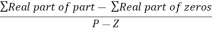
= 
Centroid = -0.66
5) As poles are complex so angle of departure
øD = (2q+1)×180°+ø
ø = ∠Z –∠P.
Calculating ø for S=0
Join all the other poles with S=0
ø = ∠Z –∠P.
= 0-(315°+45°)
= -360°
ØD = (2q + 1)180 + ø.
= 180° - 360°
ØD = -180° (for q=0)
= 180° (for q=1)
=540° (for q=2)
Calculation ØD for pole at (-1+j)

ø = ∠Z –∠P.
= 0 –(135°+90°)
= -225°
ØD = (2q+1) 180°+ø.
= 180-225°
= -45°
ØD = -45° (for q = 0)
= 315° (for q = 1)
= 675° (for q =2)
6) The crossing point on imaginary axis can be calculated by Routh Hurwitz the characteristic equation is.
1+G(s) H (s) = 0
1+
S (S2+2s+2)+k = 0
S3+2s2+2s+K = 0
For stability  > 0. And K > 0.
0<K<2.
So, when K=2 root locus crosses imaginary axis
S3 + 2S2 + 2S + 2 =0
For k
Sn-1 = 0 n: no. Of intersection
S2-1 = 0 at imaginary axis
S1 = 0
 = 0
= 0
K<4
For Sn = 0 for valve of S at that K
S2 = 0
2S2 + K = 0
2S2 + 2 = 0
2(S2 +1) = 0
32 = -2
S = ± j 
The root locus plot is shown in figure below.
Fig. Root Locus for G(S) = 
Q2. Sketch the root locus plot for the following open loop transfer function
G(s) = 
- Number of zero = 0, number of poles = 3
2. As P>Z, branches will terminates at infinity
3. There are no zeros so all branches will terminate at infinity.
4. The path for the branches is shown by asymptote
Asymptote =  ×180°. q=0,1,………p-z-1
P=3, Z=0
q= 0,1,2.
For q = 0
Asymptote =  × 180° = 60.
For q=1
Asymptote =  × 180° = 180°
For q=2
Asymptote =  × 180° = 300°
5. Asymptote intersect real axis at centroid
Centroid = 
=  = -1
= -1
6. As root locus lies between poles S= 0, and S= -1
So, calculating breakaway point.
 = 0
= 0
The characteristic equation is
1+ G(s) H (s) = 0.
1+  = 0
= 0
K = -(S3+3S2+2s)
 = 3S2+6s+2 = 0
3s2+6s+2 = 0
S = -0.423, -1.577.
So, breakaway point is at S=-0.423
Because root locus is between S= 0 and S= -1
7. The intersection of root locus with imaginary axis is given by Routh criterion.
Characteristics equation is
S3+3S3+2s+K = 0
For k
Sn-1= 0 n: no. Of intersection with imaginary axis
n=2
S1 = 0
 = 0
= 0
K < 6 Valve of S at the above valve of K
Sn = 0
S2 = 0
3S2 + K =0
3S2 +6 = 0
S2 + 2 = 0
S = ±  j
j

Fig. Root Locus for G(s) = 
The root locus plot is shown in figure.
Q4. Plot the root locus for open loop system
G(s) = 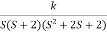
1) Number of zero = 0 number of poles = 4 located at S=0, -2, -1+j, -1-j.
2) As no zeros are present so all branches terminated at infinity.
3) As P>Z, the path for branches is shown by asymptote
Asymptote = 
q = 0,1,2……p-z-1
For q = 0
Asymptote = 45°
q=1
Asymptote = 135°
q=2
Asymptote = 225°
q=3
Asymptote = 315°
4) Asymptote intersects real axis at centroid.
Centroid = 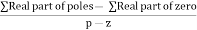
= 
Centroid = -1.
5) As poles are complex so angle of departure is
ØD=(2q+1)180° + Ø
ø = ∠Z –∠P
= 0-[135°+45°+90°]
= 180°- 270°
ØD = -90°
6) As root locus lies between two poles so calculating point. The characteristic equation is
1+ G(s)H(s) = 0
1+ = 0.
= 0.
K = -[S4+2S3+2S2+2S3+4S2+4S]
K = -[S4+4S3+6S2+4S]
 = 0
= 0
 = 4s3+12s2+12s+4=0
S = -1
So, breakaway point is at S = -1
7) Intersection of root locus with imaginary axis is given by Routh Hurwitz.
S4+4S3+6S2+4s+K = 0
 ≤ 0
≤ 0
K≤5.
For K=5 valve of S will be.
5S2+K = 0
5S2+5 = 0
S2 +1 = 0
S2 = -1
S = ±j.
The root locus is shown in figure.
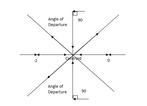
Fig. Root Locus For G(s) = 
Q5. Plot the root locus for open loop transfer function G(s) = 
- Number of zeros = 0. Number of poles = 4 located at S=0, -3, -1+j, -1-j.
2. As no. Zero so all branches terminate at infinity.
3. The asymptote shows the both to the branches terminating at infinity.
Asymptote =  q=0,1,….(p-z).
For q = 0
Asymptote = 45
For q = 1
Asymptote = 135
For q = 2
Asymptote = 225
For q = 3
Asymptote = 315
(4). The asymptote intersects real axis at centroid.
Centroid = ∑Real part of poles - ∑Real part of zero / P – Z
= [-3-1-1] – 0 / 4 – 0
Centroid = -1.25
(5). As poles are complex so angle of departure
φD = (29 + 1)180 + φ
ø = ∠Z –∠P.
= 0 – [ 135 + 26.5 + 90 ]
= -251.56
For q = 0
φD = (29 + 1)180 + φ
= 180 – 215.5
φD = - 71.56
(6). Break away point dk / ds = 0 is at S = -2.28.
(7). The intersection of root locus on imaginary axis is given by Routh Hurwitz.
1 + G(S)H(S) = 0
K + S4 + 3S3 + 2S3 + 6S2 + 2S2 + 6S = 0
S4 1 8 K
S3 5 6
S2 34/5 K
S1 40.8 – 5K/6.8
K ≤ 8.16
For K = 8.16 value of S will be
6.8 S2 + K = 0
6.8 S2 + 8.16 = 0
S2 = - 1.2
S = ± j1.09
The plot is shown in figure.

Fig. Root Locus for G(s) = 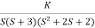
Q.6. Sketch the root locus for open loop transfer function.
G(S) = K(S + 6)/S(S + 4)
- Number of zeros = 1(S = -6)
Number of poles = 2(S = 0, -4)
2. As P > Z one branch will terminate at infinity and the other at S = -6.
3. For Break away and breaking point
1 + G(S)H(S) = 0
1 + K(S + 6)/S(S + 4) = 0
Dk/ds = 0
S2 + 12S + 24 = 0
S = -9.5, -2.5
Breakaway point is at -2.5 and Break in point is at -9.5.
4. Root locus will be in the form of a circle. So finding the centre and radius. Let S = + jw.
G( + jw) = K( + jw + 6)/( + jw)( + jw + 4 ) = +- π
Tan-1 w/ + 6 - tan-1 w/ – tan-1 w / + 4 = - π
Taking tan of both sides.
w/ + w/ + 4 / 1 – w/ w/ + 4 = tan π + w / + 6 / 1 - tan π w/ + 6
w/ + w/ + 4 = w/ + 6[ 1 – w2 / ( + 4) ]
(2 + 4)( + 6) = (2 + 4 – w2)
2 2 + 12 + 4 + 24 = 2 + 4 – w2
22 + 12 + 24 = 2 – w2
2 + 12 – w2 + 24 = 0
Adding 36 on both sides
( + 6)2 + (w + 0)2 = 12
The above equation shows circle with radius 3.46 and center(-6, 0) the plot is shown in figure.
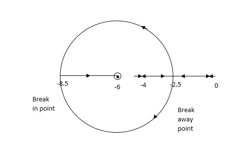
Fig. Root locus for G(S) = K (S + 6)/S (S + 4)
The plot can be used to interpret how the input affects the output in both magnitude and phase over frequency.
The Bode plot or the Bode diagram consists of two plots −
- Magnitude plot
- Phase plot
In both the plots, x-axis represents angular frequency (logarithmic scale). Whereas, y-axis represents the magnitude (linear scale) of open loop transfer function in the magnitude plot and the phase angle (linear scale) of the open loop transfer function in the phase plot.
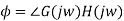
The magnitude of the open loop transfer function in dB is –
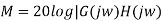
The phase angle of the open loop transfer function in degrees is
Steps for drawing bode plot
- Determine the Transfer Function of the system.
2. Rewrite it by factoring both the numerator and denominator into the standard form.
3. Replace s with j. Then find the Magnitude of the Transfer Function
If we take the log10 of this magnitude and multiply it by 20 it takes on the form of

Each of these individual terms is very easy to show on a logarithmic plot. The entire Bode log magnitude plot is the result of the superposition of all the straight-line terms. This means with a little practice; we can quickly sketch the effect of each term and quickly find the overall effect. To do this we have to understand the effect of the different types of terms.
These included:- 1. Constant term K
2. Poles and zeroes at the origin 
3. Poles and zeroes not at the origin 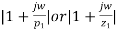
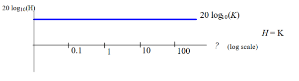
Effect of Constant Terms: Constant terms such as K contribute a straight horizontal line of magnitude 20 log10(K)
Effect of Individual Zeros and Poles at the origin: A zero at the origin occurs when there is an s or j multiplying the numerator. Each occurrence of this causes a positively sloped line passing through sj= 1 with a rise of 20 db over a decade
A pole at the origin occurs when there are s or j multiplying the denominator. Each occurrence of this causes a negatively sloped line passing through sj = 1 with a drop of 20 db over a decade
Effect of Individual Zeros and Poles Not at the Origin: Zeros and Poles not at the origin are indicated by the (1+js/zi) and (1+js/pi). The values zi and pi in each of these expressions is called a critical frequency (or break frequency). Below their critical frequency these terms do not contribute to the log magnitude of the overall plot. Above the critical frequency, they represent a ramp function of 20 db per decade. Zeros give a positive slope. Poles produce a negative slope.
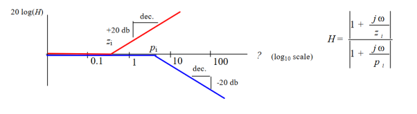
To complete the log magnitude vs. Frequency plot of a Bode diagram, we superposition all the lines of the different terms on the same plot.
Advantages and Plotting
- By looking at bode plot we can write the transfer function of system
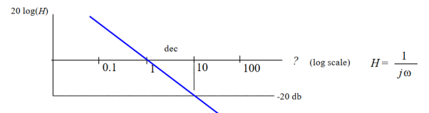
Q. G(S) = 
1. Substitute S = j
G(j ) =
) = 
M = 
 = tan-1
 = -900
Magnitude varies with ‘w’ but phase is constant.
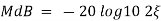
MdB = +20 log10
MdB = -20 log10
Decade frequency:
W present = 10  past
past
Then  present is called decade frequency of
  past
past
 2 = 10
  1
1
 2 is decade frequency of
  1
1
 MdB
MdB
0.01 40
0.1 20
1 0 (shows pole at origin)
0 -20
10 -40
100 -60
Slope = (20db/decade)
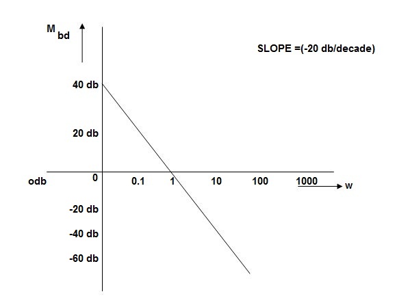
Fig. MAGNITUDE PLOT
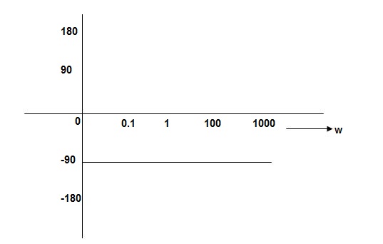
Fig. PHASE PLOT
Que. G(S) = 
Sol: G(j ) =
) = 
M =  ;
;  = -1800 (-20tan-1
 )
)
MdB = +20 log  -2
-2
MdB = -40 log10
 MdB
MdB
0.01 80
0.1 40
1 0 (pole at origin)
10 -40
100 -80
Slope = 40dbdecade
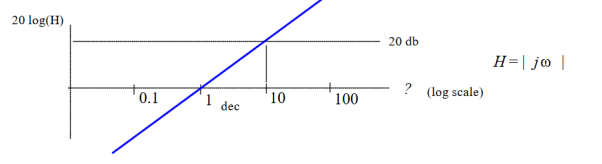
Que. G(S) = S
Sol: M= W
 = 900
= 900
MdB = 20 log10
 MdB
MdB
0.01 -40
0.1 -20
1 0
10 20
100 90
1000 60
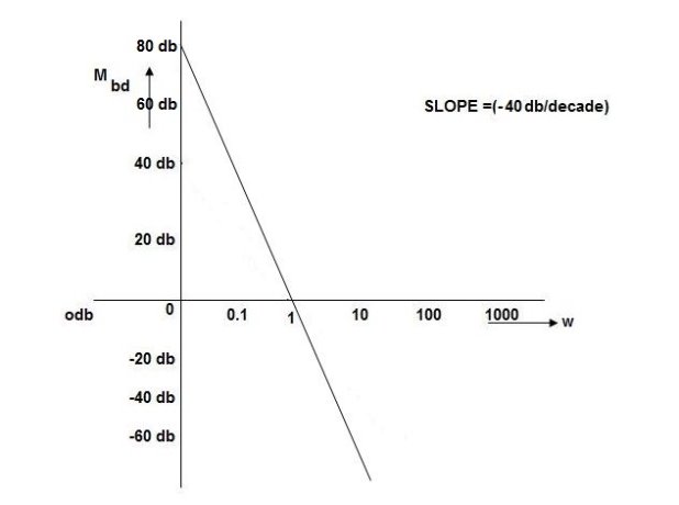
Fig. Bode Plot G(S) = S
Que. G(S) = S2
Sol: M=  2
2
MdB = 20 log10 2 == 40 log10
 = 1800
W MdB
0.01 -80
0.1 -40
1 0
10 40
100 80
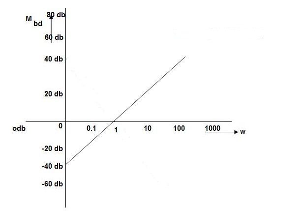
Fig. Magnitude Plot G(S) = S2
Que. G(S) = 
Sol: G(j ) =
) = 
M = 
MdB = 20 log10 K-20 log10
 = tan-1(
 ) –tan-1(
 )
)
 = 0-900 = -900
K=1 K=10
 MDb MdB
=-20 log10 =20 -20 log10
0.01 40 60
0.1 20 40
1 0 20
10 -20 0
100 -40 -20
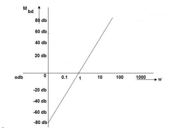
Fig. Bode Plot G(S) = 
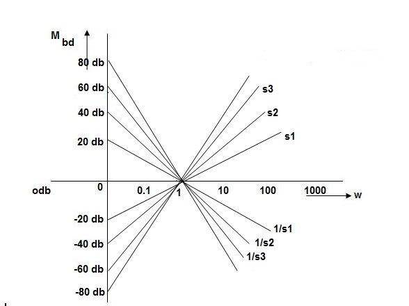
Fig. All bode plots in one plot
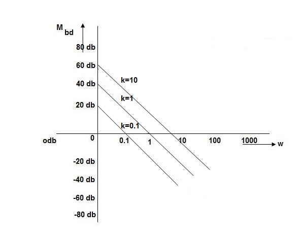
Fig. Variation in K shifts magnitude plot by +20db
As we vary K  then plot shift by 20 log10K
i.e adding a d.c. To a.c. Quantity
Approximation of Bode Plot:
If poles and zeros are not located at origin
G(S) = 
TF = 
M = 
MdB = -20 log10 (
 = -tan-1
Approximation:  T >> 1. So, we can neglect 1.
MdB = -20 log10
MdB = -20 log10 T;
T;  = -tan-1(
 T)
T)
Approximation:  T << 1. So, we can neglecting
  T.
T.
MdB= 0dB,  = 00
= 00
At a point both meet so equal i.e a time will come hence both approx become equal
-20 log10 T= 0
T= 0
 T= 1
T= 1
 corner frequency
At this frequency both the cases are equal
MdB = -20 log10
Now for 
MdB = -20 log10
= -20 log10
= -10 log102
MdB = 10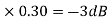
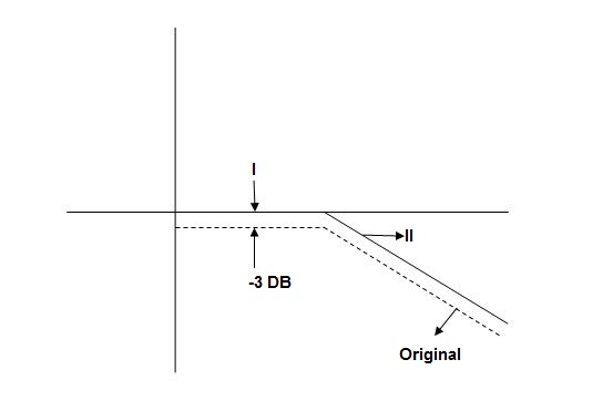
Fig. Approximation in bode plot
When we increase the value of  in app 2 and decrease the
  of app 1 so a RT comes when both cases are equal and hence for that value of
  where both app are equal gives max. Error we found above and is equal to 3dB
At corner frequency we have max error of -3dB
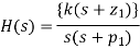
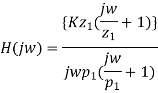
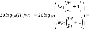
Que. G(S) = 
Sol: TF = 
M = 
MdB = -20 log10 ( at T=2
 MdB
MdB
1 -20 log10
10 -20 log10
100 -20 log10
 MdB
MdB  =
= =
= 
0.1 -20 log10 = 1.73
  10-3
10-3
0.1 -20 log10 = -0.1703
0.5 -20 log10 = -3dB
1 -20 log10 = -6.98
10 -20 log10 = -26.03
100 -20 log10 = -46.02
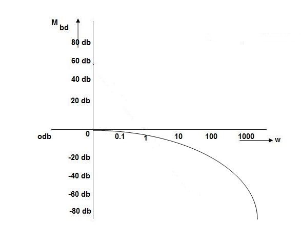
Fig. Magnitude Plot with approximation
Without approximation
For second order system
TF = 
TF = 
= 
= 
= 
M= 
MdB= 
Case 1  <<
<<
 << 1
<< 1
MdB= 20 log10 = 0 Db
Case 2  >>
>>
 >> 1
>> 1
MdB = -20 log10
= -20 log10
= -20 log10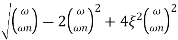
 < 1
< 1  is very large so neglecting other two terms
MdB = -20 log10
= -40 log10
Case 3. When case 1 is equal to case 2
-40 log10 = 0
= 0
 = 1
= 1

The natural frequency is our corner frequency
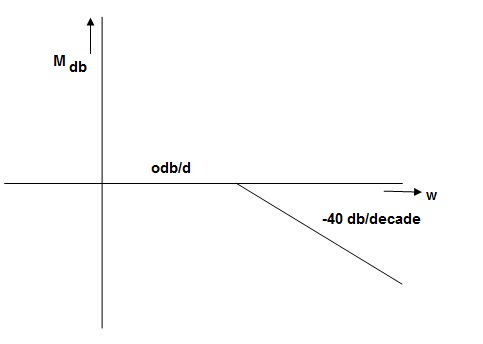
Fig. Magnitude Plot
Max error at  i.e at corner frequency
MdB = -20 log10
For 
MdB = -20 log10 
 error for
Completely the error depends upon the value of  (error at corner frequency)
The maximum error will be
MdB = -20 log10 
M = -20 log10 
 = 0
= 0

 is resonant frequency and at this frequency we are getting the maximum error so the magnitude will be
M = - +
+ 
= 
Mr =
MdB = -20 log10
MdB = -20 log10 
 = tan-1

Mr = 
Type of system | Initial slope | Intersection |
0 | 0 dB/decade | Parallel to 0 axis |
1 | -20 dB/decade | =K1 |
2 | -40 dB/decade | =K1/2 |
3 | -60 dB/decade | =K1/3 |
. | . | 1 |
. | . | 1 |
. | . | 1 |
N | -20N dB/decade | =K1/N |
Plotting
Q.1 Sketch the bode plot for transfer function
G(S) = 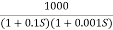
Replace S = j
G(j =
= 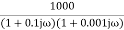
This is type 0 system . So initial slope is 0 dB decade. The starting point is given as
20 log10 K = 20 log10 1000
= 60 dB
Corner frequency  1 =
1 =  = 10 rad/sec
 2 =
2 =  = 1000 rad/sec
Slope after  1 will be -20 dB/decade till second corner frequency i.e
  2 after
  2 the slope will be -40 dB/decade (-20+(-20)) as there are poles
For phase plot
 = tan-1 0.1
 - tan-1 0.001
For phase plot


100 -900
200 -9.450
300 -104.80
400 -110.360
500 -115.420
600 -120.00
700 -124.170
800 -127.940
900 -131.350
1000 -134.420
The plot is shown in figure.

Fig. Magnitude Plot for G(S) = 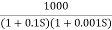
Q.2 For the given transfer function determine
G(S) = 
Gain cross over frequency phase cross over frequency phase mergence and gain margin
Initial slope = 1
N = 1, (K)1/N = 2
K = 2
Corner frequency
 1 =
1 =  = 2 (slope -20 dB/decade
 2 =
2 =  = 20 (slope -40 dB/decade

Phase
 = tan-1
 - tan-1 0.5
  - tan-1 0.05
 = 900- tan-1 0.5
  - tan-1 0.05


1 -119.430
5 -172.230
10 -195.250
15 -209.270
20 -219.30
25 -226.760
30 -232.490
35 -236.980
40 -240.570
45 -243.490
50 -245.910
Finding  gc (gain cross over frequency
M = 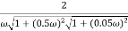
4 =  2 (
2 ( (
(
 6 (6.25
 104) + 0.252
 4 +
4 + 2 = 4
2 = 4
Let  2 = x
2 = x
X3 (6.25 104) + 0.252
 2 + x = 4
X1 = 2.46
X2 = -399.9
X3 = -6.50
For x1 = 2.46
 gc = 3.99 rad/sec(from plot)
For phase margin
PM = 1800 - 
 = 900 – tan-1 (0.5×
 gc) – tan-1 (0.05 ×
  gc)
gc)
= -164.50
PM = 1800 - 164.50
= 15.50
For phase cross over frequency ( pc)
pc)
 = 900 – tan-1 (0.5
  ) – tan-1 (0.05
  )
)
-1800 = -900 – tan-1 (0.5  pc) – tan-1 (0.05
  pc)
pc)
-900 – tan-1 (0.5  pc) – tan-1 (0.05
  pc)
pc)
Taking than on both sides
Tan 900 = tan-1
Let tan-1 0.5  pc = A, tan-1 0.05
  pc = B
 = 00
= 00
 = 0
= 0
1 =0.5  pc 0.05
 pc
pc
 pc = 6.32 rad/sec
The plot is shown in figure.

Fig. Magnitude Plot G(S) = 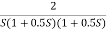
Q3. For the given transfer function
G(S) = 
Plot the rode plot find PM and GM
T1 = 0.5  1 =
1 =  = 2 rad/sec
Zero so, slope (20 dB/decade)
T2 = 0.2  2 =
2 =  = 5 rad/sec
Pole, so slope (-20 dB/decade)
T3 = 0.1 = T4 = 0.1
 3 =
3 =  4 = 10 (2 pole ) (-40 db/decade)
- Initial slope 0 dB/decade till
 1 = 2 rad/sec
2. From  1 to
1 to 2 (i.e. 2 rad /sec to 5 rad/sec) slope will be 20 dB/decade
3. From  2 to
2 to  3 the slope will be 0 dB/decade (20 + (-20))
4. From  3,
3, 4 the slope will be -40 dB/decade (0-20-20)
Phase plot
 = tan-1 0.5
 - tan-1 0.2
 - tan-1 0.1
 - tan-1 0.1


500 -177.30
1000 -178.60
1500 -179.10
2000 -179.40
2500 -179.50
3000 -179.530
3500 -179.60
GM = 00
PM = 61.460
The plot is shown in figure.
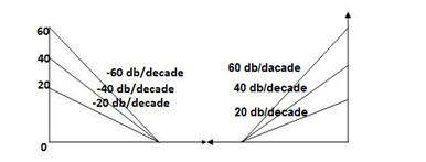
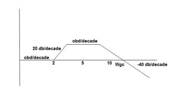

Fig. Magnitude and Phase plot for G(S) = 
Q 4. For the given transfer function plot the bode plot (magnitude plot) G(S) = 
Sol:
Given transfer function
G(S) = 
Converting above transfer function to standard from
G(S) = 
= 
- As type 1 system, so initial slope will be -20 dB/decade
2. Final slope will be -60 dB/decade as order of system decides the final slope
3. Corner frequency
T1 =  ,
,  11= 5 (zero)
T2 = 1,  2 = 1 (pole)
4. Initial slope will cut zero dB axis at
(K)1/N = 10
i.e  = 10
= 10
5. Finding  n and
n and 
T(S) = 
T(S)= 
Comparing with standard second order system equation
S2+2 ns +
ns + n2
n2
 n = 11 rad/sec
 n = 5
n = 5
 11 = 5
 =
=  = 0.27
6. Maximum error
M = -20 log 2
= +6.5 dB
7. As K = 10, so whole plot will shift by 20 log 10 10 = 20 dB
The plot is shown in figure.
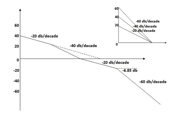
Fig. Magnitude plot for G(S) = 
Q5. For the given plot determine the transfer function
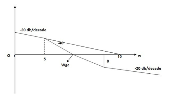
Fig. Magnitude Plot
Sol: From figure we can conclude that
- Initial slope = -20 dB/decade so type -1
2. Initial slope all 0 dB axis at  = 10 so
K1/N N = 1
(K)1/N = 10.
3. Corner frequency
 1 =
1 =  = 0.2 rad/sec
 2 =
2 =  = 0.125 rad/sec
4. At  = 5 the slope becomes -40 dB/decade, so there is a pole at
  = 5 as
Slope changes from -20 dB/decade to -40 dB/decade
5. At  = 8 the slope changes from -40 dB/decade to -20 dB/decade hence is a zero at
  = 8 (-40+(+20) = 20)
Hence transfer function is T(S) = 
Absolute stability criterion:
A stable system always gives bounded output for bounded input and the system is known as BIBO stable
A linear time invariant (LTI) system is stable if,
The system is BIBO stable
In absence of the input the output tends towards zero
For system
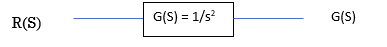
Fig. Control system with G(s) = 1/s2

For R(s) = 1
C(S) = 
R (t) =  (t) C (t) = t

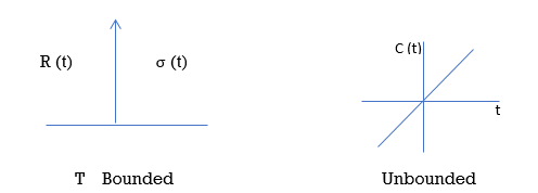
Fig. Input R(t) Fig. Input and output for 
So, system unstable.
Example 2
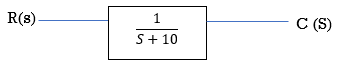
[R(s) = 1]
 =
= 
C(t) = e-10t C(t)
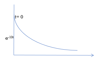
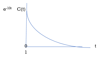
Fig. BIBO stable figure
Relative Stability Criterion:
Routh stability criterion deals about absolute stability of any closed loop system. For relative stability we need to shift the S-plane and the apply the Routh criterion.
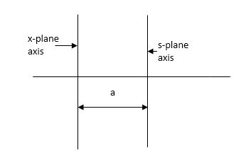
Fig. Location of Pole for relative stability
The above fig shows the characteristic equation is modified by shifting the origin of S-plane to S1= - .
.
S = Z-S1
After substituting new valve of S =(Z-S1) applying Routh stability criterion, the number of sign changes in first column is the number of roots on right half of S-plane
Gain Cross Over Frequency
The frequency at which the bode plot culls the 0db axis is called as Gain Cross Over Frequency.
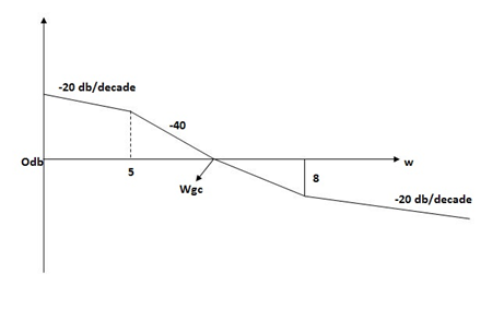
Fig. Gain cross over frequency
Phase Cross Over Frequency
The Frequency at which the phase plot culls the -1800 axis.
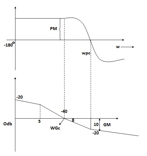
Fig. Phase Margin and Gain Margin
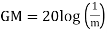
GM=MdB= -20 log [ G (jw)]
 .:
.: 
 .:
.: 
Key takeaway
i) More the difference b/WPC and WGC core are the stability of system
Ii) If GM is below 0dB axis than take +ve and stable. If GM above 0dB axis, that is take -ve GM= ODB - 20 log M
Iii) The IM should also lie above -1800 for making the system (i.e. pm=+ve
Iv) For a stable system GM and PM should be -ve
v) GM and PM both should be +ve more the value of GM and PM more the system is stable.
Vi) If Wpc and Wgc are in same line Wpc= Wgc than system is marginally stable as we get GM=0dB.
Vii) When gain cross over frequency is smaller then phase curves over frequency the system is stable and vice versa.
The transfer function of second order system is shown as
C(S)/R(S) = W2n / S2 + 2ξWnS + W2n - - (1)
ξ = Ramping factor
Wn = Undamped natural frequency for frequency response let S = jw
C(jw) / R(jw) = W2n / (jw)2 + 2 ξWn(jw) + W2n
Let U = W/Wn above equation becomes
T(jw) = W2n / 1 – U2 + j2 ξU
So,
| T(jw) | = M = 1/√(1 – u2)2 + (2ξU)2 - - (2)
T(jw) = φ = -tan-1[ 2ξu/(1-u2)] - - (3)
For sinusoidal input the output response for the system is given by
C(t) = 1/√(1-u2)2 + (2ξu)2Sin[wt - tan-1 2ξu/1-u2] - - (4)
The frequency where M has the peak value is known as Resonant frequency Wn. This frequency is given as (from eqn (2)).
DM/du|u=ur = Wr = Wn√(1-2ξ2) - - (5)
From equation(2) the maximum value of magnitude is known as Resonant peak.
Mr = 1/2ξ√1-ξ2 - - (6)
The phase angle at resonant frequency is given as
Φr = - tan-1 [√1-2ξ2/ ξ] - - (7)
As we already know for step response of second order system the value of damped frequency and peak overshoot are given as
Wd = Wn√1-ξ2 - - (8)
Mp = e- πξ2|√1-ξ2 - - (9)
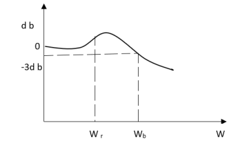
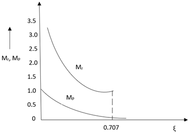
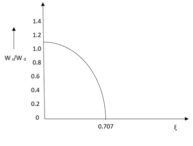
Fig. Frequency Domain Specification
The comparison of Mr and Mp is shown in figure. The two performance indices are correlated as both are functions of the damping factor ξ only. When subjected to step input the system with given value of Mr of its frequency response will exhibit a corresponding value of Mp.
Similarly the correlation of Wr and Wd is shown in fig for the given input step response [ from eqn(5) & eqn(8) ]
Wr/Wd = √(1- 2ξ2)/(1-ξ2)
Mp = Peak overshoot of step response
Mr = Resonant Peak of frequency response
Wr = Resonant frequency of Frequency response
Wd = Damping frequency of oscillation of step response.
From fig(1) it is clear that for ξ> 1/2, value of Mr does not exists.
Key takeaway
1) Mr and Mp are correlated as both are functions of the damping factor ξ only
2) When subjected to step input the system with given value of Mr of its frequency response will exhibit a corresponding value of Mp.
References:
1. I. J. Nagrath and M. Gopal, “Control Systems Engineering”, New Age International, 2009.
2. K. Ogata, “Modern Control Engineering”, Prentice Hall, 1991
3. M. Gopal, “Control Systems: Principles and Design”, McGraw Hill Education, 1997.
4. B. C. Kuo, “Automatic Control System”, Prentice Hall, 1995.


