Unit- 2
Behaviour of continuous and discrete time LTI systems
If the input to the system is unit impulse response, then the output of the system is known as impulse response of the system denoted by h(n). That is
h(n) = T [ δ(n)] …………………………………………………………. (1)
The arbitrary sequence x(n) can be represented as weighted sum of discrete impulses given by
x(n) =  δ(n-k) --------------------------------------------(2)
Then the output
y(n) = T [  δ(n-k)] -----------------------------------------------------(3)
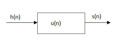
Figure 1. Step response
The step response of a discrete-time LTI system is the convolution of the unit step with the impulse response-
s[n]=u[n]*h[n]. -------------------(1)
Commutative property of convolution,
s[n]=h[n]*u[n]. ----------------------------------------(2)
That means s[n] is the response to the input h[n] of a discrete-time LTI system with unit impulse response u[n].
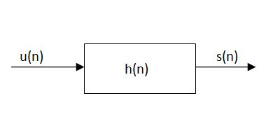
Figure 2. LTI discrete time
s[n] =  u[n-k] ------------------------------------(1)
Since u [n- k] < 0 is for n- k< 0, i.e. k> n and 1 for n -k> 0, i.e. k≤ n.
Therefore,  -----------------------------------------------(2)
That is the step response of the discrete LTI system is the running sum of its impulse response.
s[n-1] = 
s[n] – s[n-1] =  -
- 
h[n] = s[n] – s[n-1]
From here h[n] can be recovered from s[n], the impulse response of discrete-time LTI system is the first difference of its step response.
For continuous time system
The unit step response is the running integral of its impulse response.
s(t) =  ) dτ
) dτ
The unit impulse response is the first derivative of the unit step response: -
h(t) = ds(t)/dt = s’(t)
The input signal to the system is x(n) and the output is y(n).

Figure 3. I/O relation
If the input to the system is unit impulse, then the output of the system is known as impulse response of the system denoted by h(n).
h(n) = T [ ∂(n)]
The arbitrary sequence x(n) can be represented aa a weighted sum of discrete impulses given by
x(n) =  ∂(n-k)
Then the output
y(n) = T [  ∂(n-k)]
Using linear property of the system, interchange the system operator T with the summation x(k) to obtain
y(n) =  T [ ∂(n-k)]
Now
y(n) =  h(n,k)
For a time-invariant system
h(n,k) = h(n-k)
Therefore
y(n) =  h(n-k)
Thus, the output of the LTI system is given by the weighted sum of the time-shifted responses.
This sum is termed as convolution sum represented as
y(n) = x(n) * h(n) where * denotes convolution.
Problem:
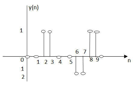
The impulse response h[n] of a discrete-time LTI system. Determine and sketch the output y[n] of this system to the input x[n]
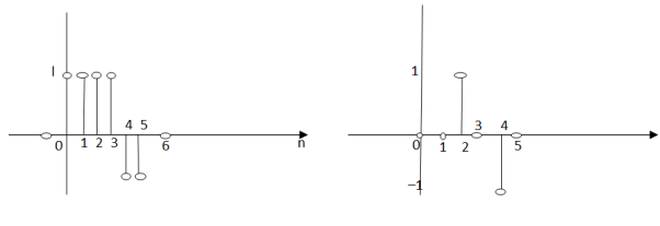
h[n] = δ[n] + δ[n-1] + δ[n-2] + δ[n-3] -δ[n-4] -δ[n-5]
x[n] = δ[n-2] -δ[n-4]
x[n] *h[n] = x[n] * { δ[n] + δ[n-1] + δ[n-2] + δ[n-3] -δ[n-4] -δ[n-5] }
= x[n] + x[n-1] + x[n-2]+x[n-3]-x[n-4]-x[n-5]
y[n] = δ[n-2] - δ[n-4] + δ[n-3] - δ[n-5] +δ[n-4] -δ[n-6] +δ[n-5] - δ[n-7] - δ[n-6] + δ[n-8] -δ[n-7] +δ[n-9]
y[n] = {0,0,1,1,0,0,-2,-2,1,1}

Key Takeaways:
Convolution is important because it relates the three signals of interest: the input signal, the output signal, and the impulse response.
If we input a periodic input signal (expressed with its Fourier Series to a stable LTI system, using superposition, we can write down the output as a second Fourier Series:

Figure.4 Periodic input signal
Where,
H(jkwo) =  e -jkwot d
Key Takeaway:
y(t) is also a Fourier Series with Fourier Series coefficients CkH(jkω0)
Consider the cascade connection of two LTI systems, as illustrated in Fig. (a). Let z(t) be the output of the first system and therefore the input to the second system in the cascade.
The output is expressed in terms of z(t) as 𝑦 (𝑡) = 𝑧(𝑡)∗ℎ2(𝑡)
Substituting for z(t), we get
y(t) =  h2(t-τ) dτ
Putting for z(t) we get
y(t) =  h1(τ-v) h2(t-τ) dv dτ
=  h(t-τ) dv
= h(t) * h(t)

Figure 5. Cascade connection
Interconnection of two LTI systems. (a) Cascade connection of two systems. (b) Equivalent system. (c) Equivalent system: Interchange system order.
Problem:
Consider the interconnection of four LTI systems as shown in figure. The impulse responses of the systems are
h1[n] = u[n]
h2[n] = u[n+2] – u[n]
h3[n] = δ[n-2]
And
h4[n] = αn u[n]
Find the impulse response h[n] of the overall system.
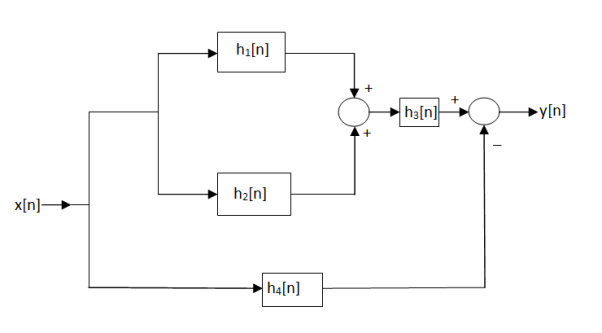
Figure6. Impulse response h[n]
We first derive the expression for the overall impulse response in the terms of impulse response of each system.
The parallel com0bination h1[n] and h2[n]. The distributive property implies that the equivalent system h12[n] = h1[n] + h2[n] as shown in figure 1.

Figure 7. Reduction
This system is in series with h3[n] so the associative property implies that the equivalent system for the upper branch has the impulse response h123[n] = h12[n] * h3[n]
Substituting for h12[n] in this expression we have
h123[n] = (h1[n] + h2[n] * h3[n]) as shown in fig(b) . Last the upper branch is in parallel with the lower branch characterized by h4[n] ; hence application of the distributive property gives the overall system impuse response as h[n] = h123[n] – h4[n]
Substituing for h123[n] in this expression yields
H[n] = ( h1[n] + h2[n] ) * h3[n] – h4[n]
As shown in fig ( c)
Now substitute the specified forms h1[n] and h2[n] to obtain
h12[n] = u[n] + u[n+2] – u[n]
=u[n+2]
Convolving h12[n] with h3[n] gives
h123[n] = u[n+2] * δ[n-2] = u[n]
Finally, we sum h123[n] and -h4[n] to obtain the overall impulse response
h[n] = {1- αn} u{n}

Figure 8. Output response
Key Takeaway:
Systems can be combined to form more complex systems otherwise known as the interconnection of systems.
Stability:
A system is said to be stable if a bounded input sequence produces bounded output sequence. For bounded input sequence x(n) if the output is unbounded the system is said to be unstable system.
Let x(n) be a bounded input sequence satisfying |x(n) | ≤ Mx < ∞. Let h(n) be the impulse response of the system then the output y(n) can be found by convolution sum. That is
y(n) =  h(n-k) = =
  x(n-k)----------------------(1)
The magnitude of the output is given by
|y(n)| = |  x(n-k)|-------------------------(2)
We know that the magnitude of the sum of terms is less than or equal to the sum of the magnitudes, hence
|y(n)| = |  x(n-k)|≤
  || x(n-k)| --------------------(3)
Let the bounded value of the input be equal to M then eq (3) can be written as
|y(n) | ≤ M  |------------------------------(4)
The above condition is satisfied when
 | < ∞ ------------------------(5)
Therefore, the necessary and sufficient condition for stability is
 | < ∞ -----------------------(6)
Therefore, the LTI system is stable if its impulse response is absolutely summable.
Causality:
If x(t) = ∂(t) then according to convolution theorem
y(t) = x(t) * h(t) = h(t) * ∂(t) = h(t)
A casual system is one where the output at the present instant does not anticipate input from future instants.
X(t) , t<to ------- y(t) , t<to
An LTI system is casual if and only if
h(t) = L (δ(t)) = 0, t<0
The impulse response of the system has to be zero for negative time for the system to be casual.
For discrete time system the impulse response of the sequence h[n] of LTI system has to be right -sided sequence
h[n] = L (δ[n]) = 0, n<0
For the given impulse response h(n) of the system determine if the system is casual or stable.
h(n) = 2 n u(-n)
The given system is non casual since h(n) ≠0 for n<0. For stability the impulse response must be absolutely summable.
 < ∞
< ∞
 n u(-n) =
  n =
n =  (1/2) n = 1+1/2 +………………. = 1/ 1-1/2 = 2
Hence system is stable
Key Takeaway:
For a LTI system to be bounded input bounded output (BIBO) stable, every bounded signal should produce a bounded output.
An LTI system is specified by equation
d 2 y(t)/ dt 2 + 5 d y(t) /dt + 6 y(t) = dx(t) / dt + 4 x(t)
The input is x(t) = e -t u(t)
Find the natural response for initial conditions:
y (0+) = 3 d y (0+)/dt =0
Forced response
Total response.
Given d 2 y(t) / dt 2 + 5 d y(t)/dt + 6 y(t) = d x(t)/dt + 4 x(t)
The natural response can be obtained by equating input terms in differential equation to zero.
d 2 y(t) / dt 2 + 5 d y(t)/dt + 6 y(t)=0
The characteristic equation is
- 2 + 5
 + 6=0
+ 6=0
- 1=-2 and
 2 = -3
The homogenous solution is
Yh(t) = c1 e -2t + c2 e -3t
y (0+) = c1 + c2
d y (0+)/dt = 2 c1 e -2t + (-3) c2 e -3t |t=0
= 2c1 – 3c2
From initial conditions
y (0+) = 3
Dy (0+)/dt =0
Comparing we get c1 + c2 =3
2c1 + 3c2 =0.
c2 =-6 and c1=9
Yn(t) = 9 e -2t – 6 e -3t
Forced response:
The homogeneous solution is given by
Yn(t) = c1 e -2t + c2 e -3t
For input x(t) = e -t
The particular solution is of the form
Yp(t) = k e -t
From which
Dyp(t)/dt = -k e-t
d2 yp(t)/dt2 = k e-t
Therefore,
d 2yp(t)/dt2 + 5 d yp(t)/dt + 6 yp(t) = dx(t)/dt + 4 x(t)
k e -t – 5 k e-t + 6 k e-t = - e-t + 4 e-t
2k = 3
K=1.5
Yp(t) = 1.5 e -t.
The forced response is the sum of homogeneous solution for particular solution.
Yf(t) = c1 e -2t + c2 e -3t + 1.5 e -t
y (0+) = c1 + c2 +1.5
Dy (0+)/dt = -2c1 e -2t -3 c2 e -3t – 1.5 e -t |t=0
To obtain forced response equate initial conditions to zero
C1 + C2 = -1.5
2C1 + 3C2 = -1.5
Solving for c1 and c2 we get
C2 = 1.5
C1 =-3
y(t) = yn(t) + yf(t)
Substituting yn(t) and yf(t) we get
y(t) = 6 e -2t – 4.5 e -3t + 1.5 e -t
y (0) = c1 + c2 + 1.5 =3
Dy (0+)/dt = -2c1 -3c2 -1.5 =0
c1 =6 and c2 =-4.5
y(t) = 6 e -2t -4.5 e -3t + 1.5 e -t
Problem:
Consider the difference equation given by
y[n] + 0.5 y[n-1] = (-0.8) n u[n]
The solution is composed of natural response and forced response of the system.
y[n] = yh[n]+yp[n]
Where the particular solution satisfies for n≥0 and the homogeneous solution satisfies
Yh[n] + 0.5 yh[n-1] = 0
For n ≥0 yp(n) = y (-0.8) n
Then we get
Y (-0.8) n + 0.5Y (-0.8) n-1 = (-0.8) n
Y [ 1+0.5(-0.8) -1] = 1
Y=8/3
Which yields yp(n) = 8/3 (-0.8) n
To determine yh(n)
Yh[n] = A z n
1+ 0.5 z -1 =0
z=-0.5
y[n] = yh[n]+yp[n] = A (-0.5) n + 8/3 (-0.8) n
y[n] = -0.5 y[n-1] + (-0.8) n u[n] -- n=0
y [0] = -0.5y [-1] + (-0.8) n =0+1=1
y [0] = 1=A (-0.5) 0 + 8/3 (-0.8) 0 = A+8/3 = 1
A=-5/3
y[n] = 5/3 (-0.5) n + 8/3 (-0.8) n
Key Takeaway:
They are used in circuit analysis, filter design, controller design, process modelling, and in many other applications.
For LTI system with output signal y(t) with input signal u(t) and impulse response h(t).
Therefore, y(t) = h(t) * u(t) -> Y(s) = H(s) U(s)
This representation of the system expresses the input output relation. It does not provide us the internal specification of the system.
State space representation not only provide information on I/O but also gives good view on the internal specification of the system.
The states of the system at time to includes min required information to express the system situation at time to. These are the first- degree equations.
State space representation of LTI system is given by
 = AX(t) + B U(t) ------ state equations
Y(t) = CX(t) + DU(t) --------- output equations
X  R n : state vector
U  R m : input vector
Y  R p : output vector
A nxn: System Matrix
B nxm: Input matrix
C pxn: Output matrix
D pxm: Coupling matrix
Number of states usually equals to degree of the system.
Set of states in not unique for the system.

Figure.9 State Space Representation
Key Takeaway:
A state-space representation is a mathematical model of a physical system as a set of input, output and state variables
The state of a dynamic system is the minimum set of variables called the state variables which if known at time to along with input the system behaviour at t>to can be determined.
A dynamic system represented by a nth- order differential equationcan be split into n first order equations which represents a state model. The model consists of chosen state variables x1, x2, xn, the input u and an output y (for single input single output system).
The state model representation of the system is
 = AX + Bu
Y= CX +Du where
X is (x1, x2, x3……………………….xn) – matrix of state variables called State matrix
A is a (nxn) matrix called Co-efficient matrix
B is a(nx1) matrix called Driving matrix
C is (1xn) matrix called Output matrix
D(nx1) matrix called Transmission matrix
U is the input and y is the output.
The state variables are the minimum set of variables. The choice of the variables in the first order equation may be different which leads to different state model of the same system.
Consider a transfer function
C(s) /R(s) = k/ (s 2 + as +b)
 + a
+ a + bc = k.r
The above equations can be written as
[ ] = [ 0 1][x1] + [0] u
[ ] = [-b -a] [x2] [k]
y [ 1 0] [ x1]
[x2]
Or
[ ] = AX + Bu
y = CX + Du
Is the state model of the second order system?
Key Takeaway:
State Space analysis also known as state variable analysis is a commonly used method nowadays for analysing the control system.
The state model of a linear, time-invariant MIMO system is a special case of the general time-invariant state model of Equations. In state representation, the derivative of each state variable can be written as a linear combination of system states and inputs i.e.
 = a11 x1(t) + a12 x2(t) + ………. + a1n xn(t) + b11 u1(t) + b12 u2(t) +…. + b1m um(t) -----------------------------------(1)
 = a21 x1(t) + a22 x2(t) + ………. + a2n xn(t) + b21 u1(t) + b22 u2(t) +…. + b2m um(t) -----------------------------------(2)
 = an1 x1(t) + an2 x2(t) + ………. +anxn(t) + bn1 u1(t) + bn2 u2(t) +…. +bnm um(t) -----------------------------------(3)
 = A x(t) + B u(t) ------ State Equation
Where x(t) =  ; State Vector
u(t) =  ; Input Vector
A =  ; System Matrix
And B =  ; Input Matrix
Similarly, the output variables can be written as a linear combination of system states and inputs that is
y1(t) = c11 x1(t) + c12 x2(t) +……..+ c1n xn(t) +d11 u1(t) + d12 u2(t) + …+ d1mum(t) ---------------------------------------(1)
y2(t) = c21 x1(t) + c22 x2(t) +……..+ c2n xn(t) +d21 u1(t) + d22 u2(t) + …+ d2mum(t)--------------------------------------------(2)
Yp(t)= cp1x1(t) + cp2x2(t) + ………. +cpnxn(t) + dp1u1(t) + dp2u2(t) +…. +dpmum(t)
Where coefficients cij = i=1,2,p; j=1,2,p: k=1,2,m are constants.
In vector form
y(t)= Cx(t) + D u(t) ---------Output Equation.
Key Takeaway:
MIMO systems that are lumped and linear can be described easily with state-space equations.
The state transition matrix is important part of both the zero input and the zero state solutions of systems represented in state space. The state transition matrix in the Laplace Domain, Φ(s), is defined as:
(s) = (s I – A)-1
Where I is the identity matrix. The time domain state transition matrix, φ(t), is simply the inverse Laplace Transform of Φ(s).
For Example,
Find Φ(s) and φ(t) if
A = 
Solution:
(s) = (s I – A)-1
= 
=
=
The inverse of a 2×2 matrix is
(s) = = =
= 
= 
To find φ(t) we must take the inverse Laplace Transform of every term in the matrix
φ(t) = ℒ-1 ((s)) = ℒ-1  = ℒ-1
= ℒ-1 
= ℒ-1 
Using partial fraction expansion of each term we get
(t) = ℒ-1 
= 
Problem:
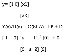
Find the transfer function for the state model given by
[ ]= [ 0 1] [x1] + [0] u(t)
[ ] [-3 -2] [x2] [2]

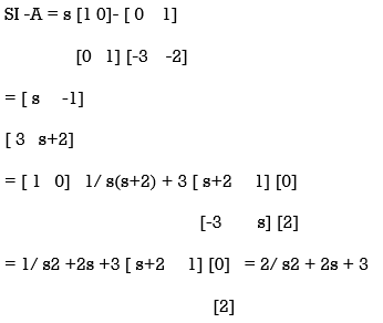
Hence T.F Y(s)/U(s) = 2/ s2 + 2s +3 given state space model.
Key Takeaway:
The state transition matrix is an important part of both the zero input and the zero state solutions of systems represented in state space.

Figure10. Periodic input to LTI system
A periodic signal with period No can be decomposed into sum of complex exponential signal
x[n] =  e j.2πk/No .n
Where,
X[k] = 1/No  e -j.2πk/No .n where k=0,………….No-1
(b) Then for each component signal
X[k] e j 2πk/No .n --- X[k] H(2πk/No) e j2πk/No.n
(c) The linearity of the filter yeilds
y[n] =  H(2πk/No) e j2πk/No.n
=  H(2πk/No) e j(2πk/No.n +
  H(2πk/No))
Key Takeaways:
When we apply a periodic input to a linear, time-invariant system, the output is periodic and has Fourier series coefficients equal to the product of the system's frequency response and the input's Fourier coefficients
The output given by the convolution sum is
y(n) =  x (n-m) --------------------------(1)
Suppose that the input is a complex exponential function, where for all n ∈ Integers, then
x(n) = e jwn ----------------------------------(2)
Then
y(n)=  ejw(n-m) -----------(3)
= e jwn e-jwm-------(4)
When the input is the complex exponential with frequency ω , then the output is given by
y(n) = H(w) e jwn -----------------------(5)
Where H(ω ) is called the frequency response.
Comparing these two expressions for the output we see that the frequency response is related to the impulse response by
H(w) =  eimw-----------(6)
H(ω ) is called the discrete-time Fourier transform (DTFT) of h(n).
Key Takeaway:
The frequency response exists if the LTI system is a stable system.
References:
- Signals and Systems by Simon Haykin
- Signals and Systems by Ganesh Rao
- Signals and Systems by P. Ramesh Babu
- Signals and Systems by Chitode
Unit- 2
Behaviour of continuous and discrete time LTI systems
If the input to the system is unit impulse response, then the output of the system is known as impulse response of the system denoted by h(n). That is
h(n) = T [ δ(n)] …………………………………………………………. (1)
The arbitrary sequence x(n) can be represented as weighted sum of discrete impulses given by
x(n) =  δ(n-k) --------------------------------------------(2)
Then the output
y(n) = T [  δ(n-k)] -----------------------------------------------------(3)

Figure 1. Step response
The step response of a discrete-time LTI system is the convolution of the unit step with the impulse response-
s[n]=u[n]*h[n]. -------------------(1)
Commutative property of convolution,
s[n]=h[n]*u[n]. ----------------------------------------(2)
That means s[n] is the response to the input h[n] of a discrete-time LTI system with unit impulse response u[n].

Figure 2. LTI discrete time
s[n] =  u[n-k] ------------------------------------(1)
Since u [n- k] < 0 is for n- k< 0, i.e. k> n and 1 for n -k> 0, i.e. k≤ n.
Therefore,  -----------------------------------------------(2)
That is the step response of the discrete LTI system is the running sum of its impulse response.
s[n-1] = 
s[n] – s[n-1] =  -
- 
h[n] = s[n] – s[n-1]
From here h[n] can be recovered from s[n], the impulse response of discrete-time LTI system is the first difference of its step response.
For continuous time system
The unit step response is the running integral of its impulse response.
s(t) =  ) dτ
) dτ
The unit impulse response is the first derivative of the unit step response: -
h(t) = ds(t)/dt = s’(t)
The input signal to the system is x(n) and the output is y(n).

Figure 3. I/O relation
If the input to the system is unit impulse, then the output of the system is known as impulse response of the system denoted by h(n).
h(n) = T [ ∂(n)]
The arbitrary sequence x(n) can be represented aa a weighted sum of discrete impulses given by
x(n) =  ∂(n-k)
Then the output
y(n) = T [  ∂(n-k)]
Using linear property of the system, interchange the system operator T with the summation x(k) to obtain
y(n) =  T [ ∂(n-k)]
Now
y(n) =  h(n,k)
For a time-invariant system
h(n,k) = h(n-k)
Therefore
y(n) =  h(n-k)
Thus, the output of the LTI system is given by the weighted sum of the time-shifted responses.
This sum is termed as convolution sum represented as
y(n) = x(n) * h(n) where * denotes convolution.
Problem:
The impulse response h[n] of a discrete-time LTI system. Determine and sketch the output y[n] of this system to the input x[n]

h[n] = δ[n] + δ[n-1] + δ[n-2] + δ[n-3] -δ[n-4] -δ[n-5]
x[n] = δ[n-2] -δ[n-4]
x[n] *h[n] = x[n] * { δ[n] + δ[n-1] + δ[n-2] + δ[n-3] -δ[n-4] -δ[n-5] }
= x[n] + x[n-1] + x[n-2]+x[n-3]-x[n-4]-x[n-5]
y[n] = δ[n-2] - δ[n-4] + δ[n-3] - δ[n-5] +δ[n-4] -δ[n-6] +δ[n-5] - δ[n-7] - δ[n-6] + δ[n-8] -δ[n-7] +δ[n-9]
y[n] = {0,0,1,1,0,0,-2,-2,1,1}
Key Takeaways:
Convolution is important because it relates the three signals of interest: the input signal, the output signal, and the impulse response.
If we input a periodic input signal (expressed with its Fourier Series to a stable LTI system, using superposition, we can write down the output as a second Fourier Series:
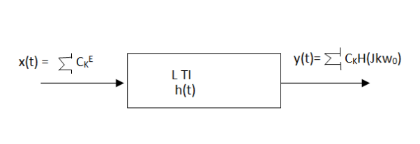
Figure.4 Periodic input signal
Where,
H(jkwo) =  e -jkwot d
Key Takeaway:
y(t) is also a Fourier Series with Fourier Series coefficients CkH(jkω0)
Consider the cascade connection of two LTI systems, as illustrated in Fig. (a). Let z(t) be the output of the first system and therefore the input to the second system in the cascade.
The output is expressed in terms of z(t) as 𝑦 (𝑡) = 𝑧(𝑡)∗ℎ2(𝑡)
Substituting for z(t), we get
y(t) =  h2(t-τ) dτ
Putting for z(t) we get
y(t) =  h1(τ-v) h2(t-τ) dv dτ
=  h(t-τ) dv
= h(t) * h(t)

Figure 5. Cascade connection
Interconnection of two LTI systems. (a) Cascade connection of two systems. (b) Equivalent system. (c) Equivalent system: Interchange system order.
Problem:
Consider the interconnection of four LTI systems as shown in figure. The impulse responses of the systems are
h1[n] = u[n]
h2[n] = u[n+2] – u[n]
h3[n] = δ[n-2]
And
h4[n] = αn u[n]
Find the impulse response h[n] of the overall system.

Figure6. Impulse response h[n]
We first derive the expression for the overall impulse response in the terms of impulse response of each system.
The parallel com0bination h1[n] and h2[n]. The distributive property implies that the equivalent system h12[n] = h1[n] + h2[n] as shown in figure 1.
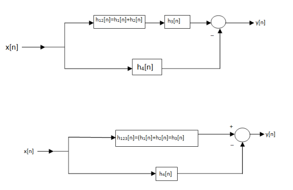
Figure 7. Reduction
This system is in series with h3[n] so the associative property implies that the equivalent system for the upper branch has the impulse response h123[n] = h12[n] * h3[n]
Substituting for h12[n] in this expression we have
h123[n] = (h1[n] + h2[n] * h3[n]) as shown in fig(b) . Last the upper branch is in parallel with the lower branch characterized by h4[n] ; hence application of the distributive property gives the overall system impuse response as h[n] = h123[n] – h4[n]
Substituing for h123[n] in this expression yields
H[n] = ( h1[n] + h2[n] ) * h3[n] – h4[n]
As shown in fig ( c)
Now substitute the specified forms h1[n] and h2[n] to obtain
h12[n] = u[n] + u[n+2] – u[n]
=u[n+2]
Convolving h12[n] with h3[n] gives
h123[n] = u[n+2] * δ[n-2] = u[n]
Finally, we sum h123[n] and -h4[n] to obtain the overall impulse response
h[n] = {1- αn} u{n}

Figure 8. Output response
Key Takeaway:
Systems can be combined to form more complex systems otherwise known as the interconnection of systems.
Stability:
A system is said to be stable if a bounded input sequence produces bounded output sequence. For bounded input sequence x(n) if the output is unbounded the system is said to be unstable system.
Let x(n) be a bounded input sequence satisfying |x(n) | ≤ Mx < ∞. Let h(n) be the impulse response of the system then the output y(n) can be found by convolution sum. That is
y(n) =  h(n-k) = =
  x(n-k)----------------------(1)
The magnitude of the output is given by
|y(n)| = |  x(n-k)|-------------------------(2)
We know that the magnitude of the sum of terms is less than or equal to the sum of the magnitudes, hence
|y(n)| = |  x(n-k)|≤
  || x(n-k)| --------------------(3)
Let the bounded value of the input be equal to M then eq (3) can be written as
|y(n) | ≤ M  |------------------------------(4)
The above condition is satisfied when
 | < ∞ ------------------------(5)
Therefore, the necessary and sufficient condition for stability is
 | < ∞ -----------------------(6)
Therefore, the LTI system is stable if its impulse response is absolutely summable.
Causality:
If x(t) = ∂(t) then according to convolution theorem
y(t) = x(t) * h(t) = h(t) * ∂(t) = h(t)
A casual system is one where the output at the present instant does not anticipate input from future instants.
X(t) , t<to ------- y(t) , t<to
An LTI system is casual if and only if
h(t) = L (δ(t)) = 0, t<0
The impulse response of the system has to be zero for negative time for the system to be casual.
For discrete time system the impulse response of the sequence h[n] of LTI system has to be right -sided sequence
h[n] = L (δ[n]) = 0, n<0
For the given impulse response h(n) of the system determine if the system is casual or stable.
h(n) = 2 n u(-n)
The given system is non casual since h(n) ≠0 for n<0. For stability the impulse response must be absolutely summable.
 < ∞
< ∞
 n u(-n) =
  n =
n =  (1/2) n = 1+1/2 +………………. = 1/ 1-1/2 = 2
Hence system is stable
Key Takeaway:
For a LTI system to be bounded input bounded output (BIBO) stable, every bounded signal should produce a bounded output.
An LTI system is specified by equation
d 2 y(t)/ dt 2 + 5 d y(t) /dt + 6 y(t) = dx(t) / dt + 4 x(t)
The input is x(t) = e -t u(t)
Find the natural response for initial conditions:
y (0+) = 3 d y (0+)/dt =0
Forced response
Total response.
Given d 2 y(t) / dt 2 + 5 d y(t)/dt + 6 y(t) = d x(t)/dt + 4 x(t)
The natural response can be obtained by equating input terms in differential equation to zero.
d 2 y(t) / dt 2 + 5 d y(t)/dt + 6 y(t)=0
The characteristic equation is
- 2 + 5
 + 6=0
+ 6=0
- 1=-2 and
 2 = -3
The homogenous solution is
Yh(t) = c1 e -2t + c2 e -3t
y (0+) = c1 + c2
d y (0+)/dt = 2 c1 e -2t + (-3) c2 e -3t |t=0
= 2c1 – 3c2
From initial conditions
y (0+) = 3
Dy (0+)/dt =0
Comparing we get c1 + c2 =3
2c1 + 3c2 =0.
c2 =-6 and c1=9
Yn(t) = 9 e -2t – 6 e -3t
Forced response:
The homogeneous solution is given by
Yn(t) = c1 e -2t + c2 e -3t
For input x(t) = e -t
The particular solution is of the form
Yp(t) = k e -t
From which
Dyp(t)/dt = -k e-t
d2 yp(t)/dt2 = k e-t
Therefore,
d 2yp(t)/dt2 + 5 d yp(t)/dt + 6 yp(t) = dx(t)/dt + 4 x(t)
k e -t – 5 k e-t + 6 k e-t = - e-t + 4 e-t
2k = 3
K=1.5
Yp(t) = 1.5 e -t.
The forced response is the sum of homogeneous solution for particular solution.
Yf(t) = c1 e -2t + c2 e -3t + 1.5 e -t
y (0+) = c1 + c2 +1.5
Dy (0+)/dt = -2c1 e -2t -3 c2 e -3t – 1.5 e -t |t=0
To obtain forced response equate initial conditions to zero
C1 + C2 = -1.5
2C1 + 3C2 = -1.5
Solving for c1 and c2 we get
C2 = 1.5
C1 =-3
y(t) = yn(t) + yf(t)
Substituting yn(t) and yf(t) we get
y(t) = 6 e -2t – 4.5 e -3t + 1.5 e -t
y (0) = c1 + c2 + 1.5 =3
Dy (0+)/dt = -2c1 -3c2 -1.5 =0
c1 =6 and c2 =-4.5
y(t) = 6 e -2t -4.5 e -3t + 1.5 e -t
Problem:
Consider the difference equation given by
y[n] + 0.5 y[n-1] = (-0.8) n u[n]
The solution is composed of natural response and forced response of the system.
y[n] = yh[n]+yp[n]
Where the particular solution satisfies for n≥0 and the homogeneous solution satisfies
Yh[n] + 0.5 yh[n-1] = 0
For n ≥0 yp(n) = y (-0.8) n
Then we get
Y (-0.8) n + 0.5Y (-0.8) n-1 = (-0.8) n
Y [ 1+0.5(-0.8) -1] = 1
Y=8/3
Which yields yp(n) = 8/3 (-0.8) n
To determine yh(n)
Yh[n] = A z n
1+ 0.5 z -1 =0
z=-0.5
y[n] = yh[n]+yp[n] = A (-0.5) n + 8/3 (-0.8) n
y[n] = -0.5 y[n-1] + (-0.8) n u[n] -- n=0
y [0] = -0.5y [-1] + (-0.8) n =0+1=1
y [0] = 1=A (-0.5) 0 + 8/3 (-0.8) 0 = A+8/3 = 1
A=-5/3
y[n] = 5/3 (-0.5) n + 8/3 (-0.8) n
Key Takeaway:
They are used in circuit analysis, filter design, controller design, process modelling, and in many other applications.
For LTI system with output signal y(t) with input signal u(t) and impulse response h(t).
Therefore, y(t) = h(t) * u(t) -> Y(s) = H(s) U(s)
This representation of the system expresses the input output relation. It does not provide us the internal specification of the system.
State space representation not only provide information on I/O but also gives good view on the internal specification of the system.
The states of the system at time to includes min required information to express the system situation at time to. These are the first- degree equations.
State space representation of LTI system is given by
 = AX(t) + B U(t) ------ state equations
Y(t) = CX(t) + DU(t) --------- output equations
X  R n : state vector
U  R m : input vector
Y  R p : output vector
A nxn: System Matrix
B nxm: Input matrix
C pxn: Output matrix
D pxm: Coupling matrix
Number of states usually equals to degree of the system.
Set of states in not unique for the system.
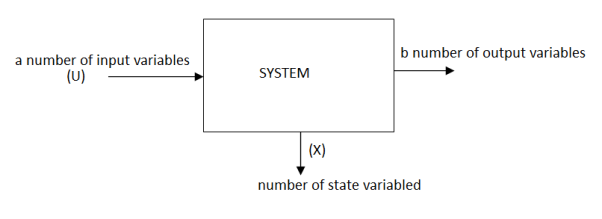
Figure.9 State Space Representation
Key Takeaway:
A state-space representation is a mathematical model of a physical system as a set of input, output and state variables
The state of a dynamic system is the minimum set of variables called the state variables which if known at time to along with input the system behaviour at t>to can be determined.
A dynamic system represented by a nth- order differential equationcan be split into n first order equations which represents a state model. The model consists of chosen state variables x1, x2, xn, the input u and an output y (for single input single output system).
The state model representation of the system is
 = AX + Bu
Y= CX +Du where
X is (x1, x2, x3……………………….xn) – matrix of state variables called State matrix
A is a (nxn) matrix called Co-efficient matrix
B is a(nx1) matrix called Driving matrix
C is (1xn) matrix called Output matrix
D(nx1) matrix called Transmission matrix
U is the input and y is the output.
The state variables are the minimum set of variables. The choice of the variables in the first order equation may be different which leads to different state model of the same system.
Consider a transfer function
C(s) /R(s) = k/ (s 2 + as +b)
 + a
+ a + bc = k.r
The above equations can be written as
[ ] = [ 0 1][x1] + [0] u
[ ] = [-b -a] [x2] [k]
y [ 1 0] [ x1]
[x2]
Or
[ ] = AX + Bu
y = CX + Du
Is the state model of the second order system?
Key Takeaway:
State Space analysis also known as state variable analysis is a commonly used method nowadays for analysing the control system.
The state model of a linear, time-invariant MIMO system is a special case of the general time-invariant state model of Equations. In state representation, the derivative of each state variable can be written as a linear combination of system states and inputs i.e.
 = a11 x1(t) + a12 x2(t) + ………. + a1n xn(t) + b11 u1(t) + b12 u2(t) +…. + b1m um(t) -----------------------------------(1)
 = a21 x1(t) + a22 x2(t) + ………. + a2n xn(t) + b21 u1(t) + b22 u2(t) +…. + b2m um(t) -----------------------------------(2)
 = an1 x1(t) + an2 x2(t) + ………. +anxn(t) + bn1 u1(t) + bn2 u2(t) +…. +bnm um(t) -----------------------------------(3)
 = A x(t) + B u(t) ------ State Equation
Where x(t) =  ; State Vector
u(t) =  ; Input Vector
A =  ; System Matrix
And B =  ; Input Matrix
Similarly, the output variables can be written as a linear combination of system states and inputs that is
y1(t) = c11 x1(t) + c12 x2(t) +……..+ c1n xn(t) +d11 u1(t) + d12 u2(t) + …+ d1mum(t) ---------------------------------------(1)
y2(t) = c21 x1(t) + c22 x2(t) +……..+ c2n xn(t) +d21 u1(t) + d22 u2(t) + …+ d2mum(t)--------------------------------------------(2)
Yp(t)= cp1x1(t) + cp2x2(t) + ………. +cpnxn(t) + dp1u1(t) + dp2u2(t) +…. +dpmum(t)
Where coefficients cij = i=1,2,p; j=1,2,p: k=1,2,m are constants.
In vector form
y(t)= Cx(t) + D u(t) ---------Output Equation.
Key Takeaway:
MIMO systems that are lumped and linear can be described easily with state-space equations.
The state transition matrix is important part of both the zero input and the zero state solutions of systems represented in state space. The state transition matrix in the Laplace Domain, Φ(s), is defined as:
(s) = (s I – A)-1
Where I is the identity matrix. The time domain state transition matrix, φ(t), is simply the inverse Laplace Transform of Φ(s).
For Example,
Find Φ(s) and φ(t) if
A = 
Solution:
(s) = (s I – A)-1
= 
=
=
The inverse of a 2×2 matrix is
(s) = = =
= 
= 
To find φ(t) we must take the inverse Laplace Transform of every term in the matrix
φ(t) = ℒ-1 ((s)) = ℒ-1  = ℒ-1
= ℒ-1 
= ℒ-1 
Using partial fraction expansion of each term we get
(t) = ℒ-1 
= 
Problem:
Find the transfer function for the state model given by
[ ]= [ 0 1] [x1] + [0] u(t)
[ ] [-3 -2] [x2] [2]

Hence T.F Y(s)/U(s) = 2/ s2 + 2s +3 given state space model.
Key Takeaway:
The state transition matrix is an important part of both the zero input and the zero state solutions of systems represented in state space.

Figure10. Periodic input to LTI system
A periodic signal with period No can be decomposed into sum of complex exponential signal
x[n] =  e j.2πk/No .n
Where,
X[k] = 1/No  e -j.2πk/No .n where k=0,………….No-1
(b) Then for each component signal
X[k] e j 2πk/No .n --- X[k] H(2πk/No) e j2πk/No.n
(c) The linearity of the filter yeilds
y[n] =  H(2πk/No) e j2πk/No.n
=  H(2πk/No) e j(2πk/No.n +
  H(2πk/No))
Key Takeaways:
When we apply a periodic input to a linear, time-invariant system, the output is periodic and has Fourier series coefficients equal to the product of the system's frequency response and the input's Fourier coefficients
The output given by the convolution sum is
y(n) =  x (n-m) --------------------------(1)
Suppose that the input is a complex exponential function, where for all n ∈ Integers, then
x(n) = e jwn ----------------------------------(2)
Then
y(n)=  ejw(n-m) -----------(3)
= e jwn e-jwm-------(4)
When the input is the complex exponential with frequency ω , then the output is given by
y(n) = H(w) e jwn -----------------------(5)
Where H(ω ) is called the frequency response.
Comparing these two expressions for the output we see that the frequency response is related to the impulse response by
H(w) =  eimw-----------(6)
H(ω ) is called the discrete-time Fourier transform (DTFT) of h(n).
Key Takeaway:
The frequency response exists if the LTI system is a stable system.
References:
- Signals and Systems by Simon Haykin
- Signals and Systems by Ganesh Rao
- Signals and Systems by P. Ramesh Babu
- Signals and Systems by Chitode