Unit - 2
Frequency transformations
The discrete Fourier transform transforms a sequence of N complex numbers  into another sequence of complex numbers
 which is defined by


Example:
Let N =4 and

Here we demonstrate how to calculate the DFT of x using equation (1)


Linear Property
If x(t) -> X(w)
Y(t) -> Y(w) then
a x(t) + b y(t) -> a X(w) +b Y(w)
Time Shifting Property
If x(t)⟷F.TX(ω)
Then Time shifting property states that
x(t−t0)⟷F.T e−jω0t X(ω)
Frequency Shifting Property
If x(t)⟷X(ω)
Then frequency shifting property states that
Ejω0t.x(t)⟷X(ω−ω0)
Time Reversal Property
If x(t)⟷X(ω)
Then Time reversal property states that
x(−t)⟷X(−ω)
Differentiation Property
If x(t)⟷X(ω)
Then Differentiation property states that
Dx(t)dt⟷jω.X(ω)
dnx(t)dtn⟷(jω)n.X(ω)
Integration Property
Integration property states that
∫x(t)dt⟷1jω X(ω)
Then
∭...∫x(t)dt⟷(jω)n X(ω)
Multiplication and Convolution Properties
If x(t)⟷X(ω)
y(t)⟷Y(ω)
Then multiplication property states that
x(t).y(t)⟷X(ω)∗Y(ω)
And convolution property states that
x(t)∗y(t)⟷1/2πX(ω).Y(ω)
Numericals:
- Compute the N-point DFT of x(n)=3δ(n).


2. Compute the N-point DFT of x(n)=7(n−n0)
Solution − We know that,

Substituting the value of x(n),

Let us take two finite duration sequences  ,having integer length as N. Their DI are
  reapectively which is shown below


Now we will try to find the DFT of another sequence  , which is given by

By taking the IDFT of the above we get

After solving the above equation finally we get

Methods of Circular Convolution
Generally, there are two methods, which are adopted to perform circular convolution and they are −
- Concentric circle method,
- Matrix multiplication method.
Concentric Circle Method
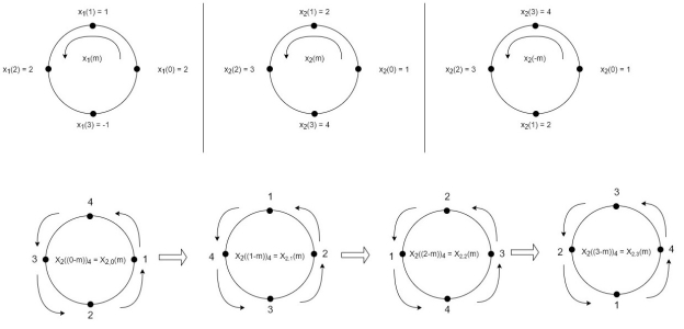
Let x1(n) and x2(n) be two given sequences. The steps followed for circular convolution of x1(n) and x2(n) are
- Take two concentric circles. Plot N samples of x1(n) on the circumference of the outer circle maintaining equal distance successive points maintaining equal distance successive points in anti-clockwise direction.
- For plotting x2(n), plot N samples of x2(n) in clockwise direction on the inner circle, starting sample placed at the same point as 0th sample of x1(n)
- Multiply corresponding samples on the two circles and add them to get output.
- Rotate the inner circle anti-clockwise with one sample at a time.
Matrix Multiplication Method
Matrix method represents the two given sequence x1(n) and x2(n) in matrix form.
- One of the given sequences is repeated via circular shift of one sample at a time to form a N X N matrix.
- The other sequence is represented as column matrix.
- The multiplication of two matrices give the result of circular convolution.
Numerical:
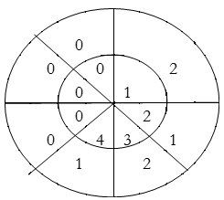
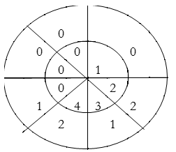
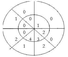
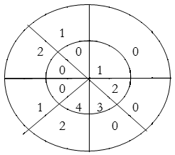
Perform circular convolution of the two sequences, x1(n)= {2,1,2,-1} and x2(n)= {1,2,3,4}

(2)

When n=0;


The sum of samples of v0(m) gives x3(0)
⸫ x3(0)=2+4+6-2=10
When n=1; 


The sum of samples of v1(m) gives x2(1)
⸫ x3(1)=4 + 1 +8-3=10
(3) When n=2; 


The sum of samples of v2(m) gives x3(2)
⸫ x3(2)=6+2+2-4=6
(4) When n=3; 


The sum of samples of v3(m) gives x3(3)
⸫ x3(3)=8+ 3+ 4-1= 14
x3(n)={10,10,6,14}


= x1(0) x x2,0(0) + x1(1) x2,0(1) + x1(2) x2,0(2) + x1(3) x2,0(3)
= 2 x 1 + 1 x 4 + 2 x 3 + (-1) x 2 = 2 +4 +6 -2 =10
Computation of linear convolution using circular convolution
Find circular convolution and linear using circular convolution for the following sequences x1(n) = {1, 2, 3, 4} and x2(n) = {1, 2, 1, 2}. Using Time Domain formula method.
Solution:
Circular convolution using circular convolution:
x1x1(n) = {1, 2, 3, 4}
And x2x2 (n) = {1, 2, 1, 2}
L=4, M=4
Length of y(n) = L+M-1=4+4-1=7
∴,x1(n) = {1, 2, 3, 4, 0, 0, 0}
& x2(n) = {1, 2, 1, 2, 0, 0, 0}
For y(0),
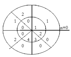
∴ y(0)= 1×1=1
For y(1),
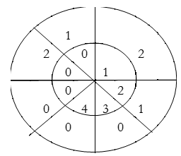
∴ y(1)= 2×1+1×2=4
For y(2),
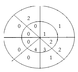
∴ y(2)= 1×1+2×2+3×1=8
For y(3),
y(3)=1×2+2×1+3×2+4×1=14
For y(4),
∴ y(4)= 4×2+3×1+2×2=15
For y(5),
∴ y(5) = 4×1+3×2=10
For y(6),
∴ y(6) = 4×2=8
∴y(n) = {1, 4, 8, 14, 15, 10, 8}
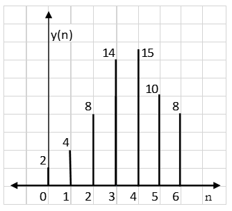
Result: y(n) = {2, 4, 8, 14, 15, 10, 8}
Linear using circular convolution:
For y(0),
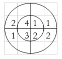
∴ y(0)= 1+4+3+8=16
For y(1),
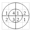
∴ y(1)= 2+2+6+4=14
For y(2),
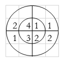
∴ y(2)= 1+4+3+8=16
For y(3),
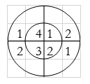
∴ y(3)= 2+2+6+4=14
y(n) = {16, 14, 16, 14}
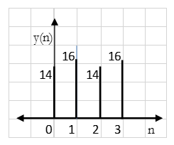
Result: y(n) = {14, 16, 14, 16}
Linear Convolution states that
y(n) = x(n) * h(n)


Example 1: h(n) = { 1 , 2 , 1, -1 } & x(n) = { 1, 2, 3, 1 } Find y(n).
METHOD 1: GRAPHICAL REPRESENTATION
Step 1) Find the value of n = nx+ nh = -1 (Starting Index of x(n)+ starting index of h(n))
Step 2) y(n)= { y(-1) , y(0) , y(1), y(2), ….} It goes up to length(xn)+ length(yn) -1. i.e n=-1


METHOD 2: MATHEMATICAL FORMULA
Use Convolution formula

k= 0 to 3 (start index to end index of x(n))
y(n) = x(0) h(n) + x(1) h(n-1) + x(2) h(n-2) + x(3) h(n-3)
METHOD 3: VECTOR FORM (TABULATION METHOD)
X(n)= {x1,x2,x3} & h(n) ={ h1,h2,h3}
|  |  |  |
 |  |  |  |
 |  |  |  |
 |  |  |  |
y(-1) = h1 x1
y(0) = h2 x1 + h1 x2
y(1) = h1 x3 + h2x2 + h3 x1 …………
METHOD 4: SIMPLE MULTIPLICATION FORM


Usually, we calculate N point DFT as N is an important factor. It can also be considered as N= r1, r2, r3, …… rv
r is selected because it represents Radix of FFT algorithm.
N = rv
For instance, if N= 8 and r =2 we can write
N = rv = 2v
8=2v
v= 3
v represents the number of stages in the FFT algorithm. But in signal processing we only relate to the number of samples. For DFT we select number of samples N and we divide by r. For example
Let N= 8
N’ = N/2 =4
N’ is still divisible by 2. N’=N/2=4/2 =2
Now N’’=r=2 and stop the process.
Decimation-in-time algorithm
This algorithm is known as Radix-2 DIT-FFT algorithm which means the number of output points N can be expressed as a power of 2 that is N = 2M where M is an integer.
Let x(n) be a sequence where N is assumed to be a power of 2. Decimate or break this sequence into two sequences of length N/2 where one sequence consists of even-indexed values of x(n) and the other of odd-indexed values of x(n).
Xe(n) = x(2n) n= 0,1,……….. N/2-1
Xo(n) = x(2n+1) n= 0,1,……….. N/2 -1
The N-pt DFT of x(n) can be written as
X(k) =  WN nk where k=0,1……….. N-1.
Separating x(n) into even and odd indexed values of x(n) we obtain
X(k) =  WN nk +
  WN nk
WN nk
( n even) (n odd)
=  WN 2nk +
  WN (2n+1)k
=  WN 2nk + Wnk
  W N 2nk
X(k) =  WN 2nk + Wnk
  W N 2nk
WN2 =( e-j2π/N) 2 = e-j2π/N/2 = W N/2 .
WN2 = W N/2
X(k) =  W N/2n k + WNk
  WN/2kn
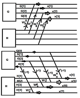
W84 = -1
W8 5 = - W 81
W86 = - W82
W87 = - W83
G(0) – H(0) = x(4)
G(1) - W 81 H(1) = x(5)
G(2) - W82 H(2) = x(6)
G(3) - W83 H(3) = x(7)
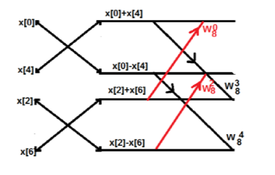
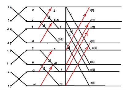
Consider the sequence x[n]={ 2,1,-1,-3,0,1,2,1}. Calculate the FFT.
Arrange the sequence as x(0) x(4) x(2) x(6) x(1) x(5) x(3) x(7)
Since N=8 find the values W8 0 to W 87
Apply the butterfly diagram to obtain the values.
Decimation in Frequency FFT
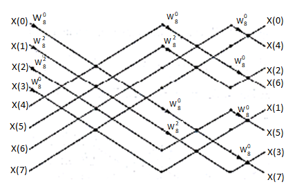
Apart from time sequence, an N-point sequence can also be represented in frequency. Let us take a four-point sequence to understand it better.
Let the sequence be x[0],x[1],x[2],x[3]………..x[7]
Mathematically, this sequence can be written as;
X(k) =  WN n-k where k=0,1……….. N-1.
Now let us make one group of sequence number 0 to 3 and another group of sequence 4 to 7. Now, mathematically this can be shown as
=  WN nk +
  WN nk
WN nk
Let us replace n by r, where r = 0, 1 , 2….N/2−1.
=  W N/2 nr
We take the first four points x[0],x[1],x[2],x[3] initially, and try to represent them mathematically as follows –
 W 8 nk +
  W8 (n+4) k
=  +
+  W8 (n+4) k
=  + {
+ {  W8 (4) k } W8 nk
X[0] =  + X[n+4]
X[1] =  + X[n+4]) W8 nk
= X(0) – X(4) + (x[1] – X[5]) W8 1 + ( X[2] – X[6] )W82 + X(3) – X(7) W8 3
DIF –FFT Algorithm
Find the DIF –FFT of the sequence x(n)= { 1,-1,-1,1,1,1,-1} using Dif-FFT algorithm.
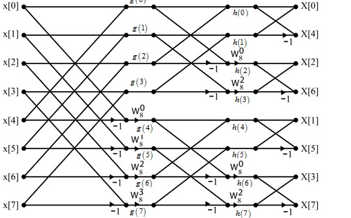
X(0)= 20 X(4) =0
X(1) = -5.828- j2.414 X(5) = -0.1716 + j 0.4141
X(2) = 0 X(6) = 0
X(3) = -0.171 – j 0.4142 X(7) = -5.8284 + j2.4142
The two methods used for filtering long sequences to short sequence are
Overlap-Save Method
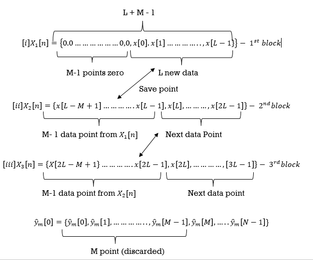
The below figure shows this method. The steps involved are
- Size of data input block is N =L+M-1
- Size of DFT and IDFT are of length N
- Input data sequence is segmented into block of L points
- FIR filter response has duration M
- L>>M which means data sequence is longer than impulse response
- As length is L+M-1 data points in impulse response are increased in length by appending L-1 zeros
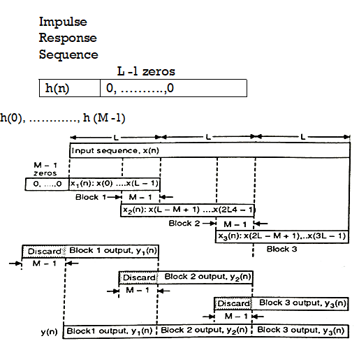
Fig: Overlap-Save Method
- Each data block consists of last M-1 data points of previous data block and L data points from data sequence follows it
- Multiplication of two N point DFT H[k] and Xm[k] for mth block of data
 [k] = H[k] Xm[k] for 0≤ k ≤ N-1
- N point DFT will be given as
 [n] = {ym(0), ym(1),…. ym(N-1)}
- Data record is of length N therefore, first M-1 points of ym[n] are corrupted by aliasing and must be discarded. The last L points are exactly same as result from linear convolution.
 =ym[n]
- To avoid loss of data due to aliasing last M-1 points of each data records are saved. The saved M-1 points become first M-1 data points of subsequent record. Initially M-1 points of first record are set to 0.
Example
The unit sample response sequence of a system h[n] = {3,2,1}. Use the overlap save method to determine its output sequence in response to the repeating input sequence {2,0,-2,0,2,1,0,-2,-1,0}. Take N=8.
Sol:
- h[n] = {3,2,1}, M=3, M-1 =2
- x[n] = {2,0,-2,0,2,1,0,-2,-1,0}
- If N = L+M-1= L+3-1
8=L+2
L=6
The length of block selected is 6.
 | -2 | -1 | 0 | 1 | 2 | 3 | 4 | 5 | 6 | 7 | 8 | 9 | 10 | 11 | … |
 |
|
| 2 | 0 | -2 | 0 | 2 | 1 | 0 | -2 | -1 | 0 | 2 | 0 | … |
 |
| 0) | 2 | 0 | -2 | 0 | 2 | 1 |
|
|
|
|
|
|
|
 |
|
|
|
|
|
| 2 | 1 | 0 | -2 | -1 | 0 | 2 | 0 |
|
 |
|
|
|
|
|
|
|
|
|
|
|
| 2 | 0 | … |
 Block 1
  Zeros added
 Block 2
 Block 3
- Pad L-1 zeros to h[n]. Therefore, sequence will be
h[n] = {3,2,1,0,0,0,0,0}
- Perform circular convolution of h[n] with x1[n] which is shown below
| Periodic extension of data block 1 | Data block 1 | ||||||||||||||
 | 0 | 2 | 0 | -2 | 0 | 2 | 1 | 0 | 0 | 2 | 0 | -2 | 0 | 2 | 1 | |
 | 0 | 0 | 0 | 0 | 0 | 1 | 2 | 3 |  |
|
|
|
|
|
| |
 |
|
|
|
|
|
|
| 4 | 1 | 6 | 4 | -4 | 4 | 4 | 7 | |
- Take block 2 and circular convolve with h[n] as shown below
| Periodic extension of data block 2 | Data block 2 | ||||||||||||||
 | 1 | 0 | -2 | -1 | 0 | 2 | 0 | 2 | 1 | 0 | -2 | -1 | 0 | 2 | 0 | |
 | 0 | 0 | 0 | 0 | 0 | 1 | 2 | 3 |  |
|
|
|
|
|
| |
 |
|
|
|
|
|
|
| 8 | 7 | 4 | -5 | -7 | 4 | 5 | 4 | |
- Add y1[n], y2[n] and so on but discard first two values from the answer and save last six values of each circular convolution as shown in figure below.
 | -2 | -1 | 0 | 1 | 2 | 3 | 4 | 5 | 6 | 7 | 8 | 9 | 10 | 11 | … |
 | 4 | 1 | 6 | 4 | -4 | -4 | 4 | 7 |
|
|
|
|
|
|
|
 |
|
|
|
|
|
| 8 | 7 | 4 | -5 | -7 | -4 | 5 | 4 |
|
 |
|
|
|
|
|
|
|
|
|
|
|
| X | X | … |
 |
|
| 6 | 4 | -4 | -4 | 4 | 7 | 4 | -5 | -7 | -4 | 5 | 4 | … |
Final answer from overlap save method
Overlap-Add Method
- Size of input data block is L points.
- Size of DFT and IDFT is N = L+M-1
- To data block we append M-1 zeros as shown below.
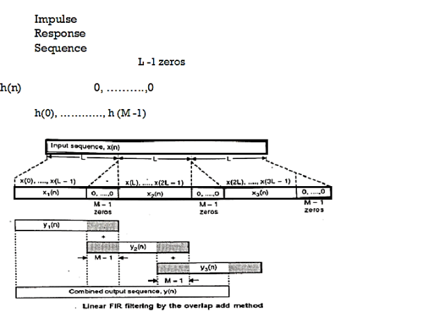
Fig: Linear FIR Filtering by overlap add method
After multiplying impulse response of length of M with DFT of input sequence we get
Ym[k] = H[k] Xm[k]
Taking IDFT of Ym[k]. The output of IDFT is block of length M
N= L+M-1. The M-1 points from each output block must overlap and should be added to first M-1 points of succeeding block. The output sequence is given by
y1[n] = y1[0], y1[1],….y1[L-1],y1[L],y1[L+1]……..y1[L+M-1]
y2[n] = y2[0], y2[1],….y2[L-1],y2[L],y2[L+1]……..y2[L+M-1]
y[n] = y[0],y[1],……y[L-1],y[L],y[L+1]……..y[L+M-1]
Example
The unit sample sequence of a system is h[n] = {3,2,1}. Use overlap add method to determine its output sequence in response to the repeating input sequence {2,0,-2,0,2,1,0,0,-2,-1,0}. Take N=8.
Sol:
- h[n] = {3,2,1}, M=3, M-1 =2
- x[n] = {2,0,-2,0,2,1,0,-2,-1,0}
- If N = L+M-1= L+3-1
8=L+2
L=6
From input every time 6 elements are selected and two zeros (M-1) are padded after them as shown below.
 | 0 | 1 | 2 | 3 | 4 | 5 | 6 | 7 | 8 | 9 | 10 | 11 | 12 | 13 | … |
|
 | 2 | 0 | -2 | 0 | 2 | 1 | 0 | -2 | -1 | 0 | 2 | 0 | -2 | 0 | … |  |
 | 2 | 0 | -2 | 0 | 2 | 1 | 0 | 0 |
|
|
|
|
|
|
|  |
 |
|
|
|
|
|
| 0 | -2 | -1 | 0 | 2 | 0 | 0 | 0 |
|  |
 |
|
|
|
|
|
|
|
|
|
|
|
| -2 | 0 | … |  |
Breaking up long input sequence into blocks of data
- Pad L-1 zeros to h[n] sequence. Therefore, sequence will be
h[n] = {3,2,1,0,0,0,0,0}
- Perform circular convolution of h[n] with x1[n] which is shown below
| Periodic extension of data block 1 | Data block 1 |
| ||||||||||||||||
 | 0 | -2 | 0 | 2 | 1 | 0 | 0 | 2 | 0 | -2 | 0 | 2 | 1 | 0 | 0 |  | |||
 | 0 | 0 | 0 | 0 | 0 | 1 | 2 | 3 |  |
|
|
|
|
|
|   | |||
 |
|
|
|
|
|
|
| 6 | 4 | -4 | -4 | 4 | 7 | 4 | 1 |  | |||
- Now circular convolution is performed for h[n] and x2[n] as shown below.
| Periodic extension of data block 2 | Data block 2 | ||||||||||||||
 | -2 | -1 | 0 | 2 | 0 | 0 | 0 | 0 | -2 | -1 | 0 | 2 | 0 | 0 | 0 | |
 | 0 | 0 | 0 | 0 | 0 | 1 | 2 | 3 |  |
|
|
|
|
|
| |
 |
|
|
|
|
|
|
| 0 | -6 | -7 | -4 | 5 | 4 | 2 | 0 | |
- Do circular convolution of h[n] with different data blocks. After performing this for all we need to add up all the outputs y1[n], y2[n] and so on.
- While considering all the output sequences we do not discard any values and just keep on adding up the overlapped area as shown below.
 | -2 | -1 | 0 | 1 | 2 | 3 | 4 | 5 | 6 | 7 | 8 | 9 | 10 | 11 | … |
 | 6 | 4 | -4 | -4 | 4 | 7 | 4 | 1 |
|
|
|
|
|
|
|
 |
|
|
|
|
|
| 0 | -6 | -7 | -4 | 5 | 4 | 2 | 0 |
|
 |
|
|
|
|
|
|
|
|
|
|
|
| X | X | … |
 | 6 | 4 | -4 | -4 | 4 | 7 | 4 | -5 | -7 | -4 | 5 | 4 | X | X | … |
Final answer from overlap add method
Key takeaway
Overlap-Save Method
- Size of data input block is N =L+M-1
- Size of DFT and IDFT are of length N
- Input data sequence is segmented into block of L points
- FIR filter response has duration M
- L>>M which means data sequence is longer than impulse response
- As length is L+M-1 data points in impulse response are increased in length by appending L-1 zeros
Image Transforms
- Many times, image processing tasks are best performed in that of a domain other than the spatial domain.
- Key steps:
(1) Transform the image
(2) Carry the task(s) in the transformed domain.
(3) Apply inverse transform to return to the spatial domain

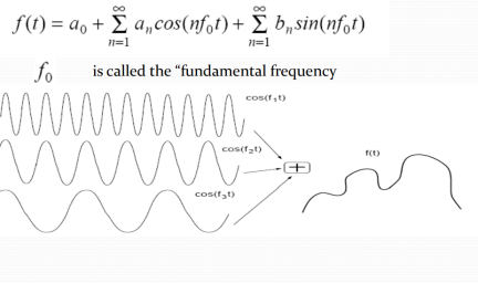
Fourier series Theorem
Any periodic function f(t) can be expressed as a weighted sum (infinite) of sine and
Discrete Fourier Transform (DFT)
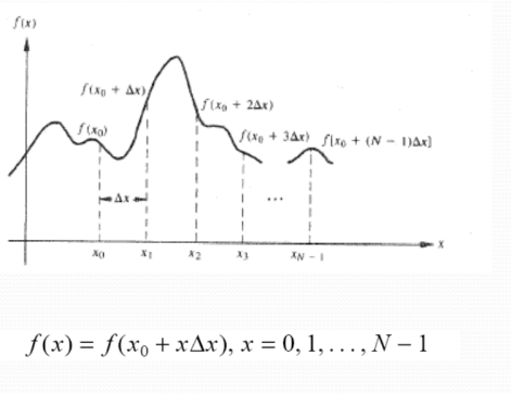
Forward DFT

Inverse DFT

Discrete Cosine Transform
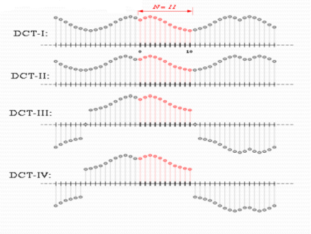
A discrete cosine transform (DCT) expresses as a finite sequence of that of the data points in terms of a sum of cosine functions oscillating at the different frequencies.
DCT is a Fourier-related transform same as that of the discrete Fourier transform (DFT), but using only real numbers. DCTs are equivalent to DFTs of roughly twice the length, operating on the real data with even symmetry. Types of DCT are listed below with eleven samples.
Key takeaway
Many times, image processing tasks are best performed in that of a domain other than the spatial domain.
Discrete Cosine Transform (DCT) is an important technique or method to convert a signal into elementary frequency component. It is widely used in image compression techniques like in JPEG compression. It converts each pixel value of an image into its corresponding frequency value. The present paper deals with the study of transformation of an 8 bit (b/w) image into its frequency domain through DCT technique.
References:
1. Ifeachor E.C, Jervis B. W, “Digital Signal Processing: Practical approach”, Pearson Publication, 2nd Edition.
2. Li Tan, “Digital Signal Processing: Fundamentals and Applications”, Academic Press, 3rd Edition.
3. Schaum's Outline of “Theory and Problems of Digital Signal Processing”, 2nd Edition.
4. Oppenheim, Schafer, “Discrete-time Signal Processing”, Pearson Education, 1st Edition.
5. K.A. Navas, R. Jayadevan, “Lab Primer through MATLAB”, PHI, Eastern Economy Edition.

