Unit - 6
Viscous Flow
A fluid can flow in a pipe in either a laminar or turbulent manner. Osborne Reynolds 11842–19122, a British physicist and mathematician, was the first to use a simple device to distinguish between these two types of flow.
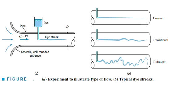
By injecting neutrally buoyant dye into a pipe with a diameter D and an average velocity V, the following features can be observed. The dye streak 1a streakline2 will flow along as a well-defined line with only little blurring owing to molecular diffusion of the dye into the surrounding water at "small enough flowrates." The dye streak swings in time and space at a slightly higher "intermediate flowrate," and intermittent bursts of abnormal behaviour develop along the streak.
For "big enough flowrates," on the other hand, the dye stripe blurs almost instantly and spreads randomly across the whole pipe. Laminar, transitional, and turbulent flow are the three characteristics.
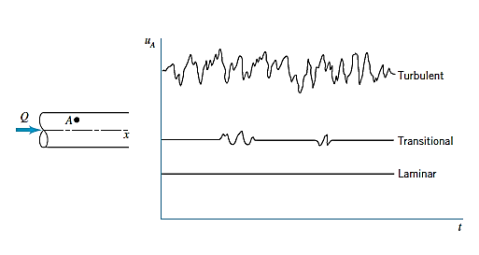
The graphs depicting the x component of velocity as a function of time at point A in the flow are presented below. The dye is dispersed throughout the pipe and causes the blurred look due to the random fluctuations of the turbulent flow (and the related particle mixing). There is only one component of velocity in laminar flow in a conduit.

The primary component of velocity in turbulent flow is also along the pipe, but it is unsteady (random), and it is accompanied by random components normal to the pipe axis.

In a typical flow, such motion is too quick for our eyes to keep up with. Slow motion images of the flow can illustrate the flow's uneven, unpredictable, and chaotic nature more clearly.
Only in relation to a reference quantity is a quantity "big" or "little." The product of these two quantities is a dimensionless quantity. The Reynolds number, Re—the ratio of inertia to viscous effects in the flow—is the most essential dimensionless parameter for pipe flow. As a result, Reynolds number should be used instead of flowrate.

That is, if the Reynolds number is "little enough," "middle," or "big enough," the flow in a pipe is laminar, transitional, or turbulent. The density, viscosity, and pipe size are all important factors in determining the flow's nature. The Reynolds number is the result of combining these parameters. Osborne Reynolds initially identified the difference between laminar and turbulent pipe flow, as well as the need of a dimensionless quantity, in 1883.
It's impossible to say exactly what Reynolds number ranges produce laminar, transitional, or turbulent pipe flows. Depending on how much the flow is disrupted by pipe vibrations, roughness of the entrance region, and other factors, the transition from laminar to turbulent flow can occur at various Reynolds numbers.
If the Reynolds number in a round pipe is less than 2100, the flow is laminar. If the Reynolds number is more than 4000, the flow through a round pipe is turbulent. The flow may vary between laminar and turbulent conditions in an apparently random manner for Reynolds values between these two boundaries (transitional flow).
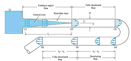
Key Takeaway:


The velocity distribution throughout a segment, the ratio of maximum velocity to average velocity, the shear stress distribution, and pressure drop for a given length must all be determined for the flow of viscous fluid via circular pipe. If the Reynolds number (Re *) is less than 2000, the flow through the circular pipe will be viscous or laminar.


Pressure Intensity on Face AB

Pressure on Face CD

Pressure force on Face AB

Pressure force on Face CD

Shear force on the surface of fluid element

As , there is no acceleration, hence the summation of all forces in the direction of flow must be zero,


Velocity Distribution:

In this equation, the distance y is measured from the boundary. The radial distance r is related to distance y by the relation.


Integrating the above equation w. r. t. ‘r’ we get

Where C is the constant of integration, and its value is obtained from the boundary conditions.
At r = R, u = 0


So,


Ratio of Maximum velocity to average velocity:
The velocity is maximum when r = 0

The fluid flowing per second through this elementary ring:


So, Average velocity,

So,

Drop of pressure for a given Length (L) of a pipe,

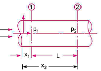

Integrating,


Loss of pressure head,


Key Takeaway:


The shear stress distribution, velocity distribution across a segment, ratio of maximum velocity to average velocity, and pressure head differential for a certain length of parallel plates must all be computed in this scenario.
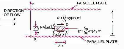
Pressure Intensity on Face AB

Pressure on Face CD

Shear stress  acting on the face BC then the shear stress on the face AD

If the width of the element in the direction perpendicular to the paper is unity, then the forces acting on the fluid element are:


So,
There is no acceleration in a steady and uniform flow, hence the resultant force in the flow direction is zero.


Velocity Distribution:


Integrating:


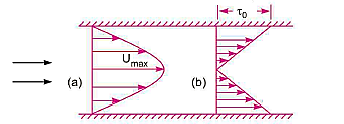
Ratio of Maximum Velocity to Average Velocity:


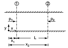
Drop of pressure head for a given Length:


Integrating:



Shear stress distribution:


Key Takeaway:


Footstep Bearing:
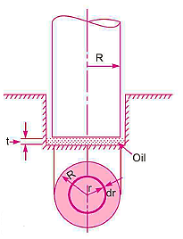


Area of the elementary ring,

Shear Stress,


Shear force on the ring,


Torque required to overcome the viscous resistance,


Total torque required to overcome the viscous resistance


Power absorbed:


Collar Bearing:
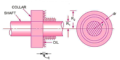


Power absorbed:


Key Takeaway:


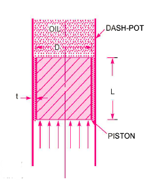


The viscous flow between two parallel plates is analogous to the flow of oil through clearance. The pressure differential between parallel plates of length 'L' is given by

The difference of pressure at the two ends of piston is given by:

So,


V is the velocity of piston or the velocity of oil in dashpot in contact with piston. The rate of flow of oil in dashpot.


Rate of flow through clearance = velocity through clearance x area of clearance

Applying continuity equation,


So,


Key Takeaway:

Capillary Tube Method:
The viscosity of a liquid is estimated using the capillary tube method by measuring the pressure differential across a certain length of capillary tube. Calculating viscosity is done using the Hagen Poiseuille law. A constant head tank is filled with the liquid whose viscosity is to be determined. The liquid is kept at a constant temperature and permitted to travel from the constant head tank through the capillary tube. The liquid is then collected in a measuring tank for a set period of time. The rate at which liquid is gathered in the tank per second is then calculated. The pressure head, abbreviated as 'h,' is measured at a distance from the tank.
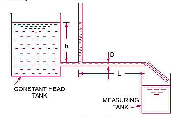

The pressure at outlet is atmospheric


Using Hagen Poiseuille's Formula,

But,

So,


Falling Sphere Method:
Falling sphere method of measuring viscosity of a liquid is based on Stokes law. A small spherical ball is released into the liquid to be tested and it accelerate under the gravitational force until it reaches a maximum terminal velocity V when the buoyant and viscous drag forces balance the gravity force.
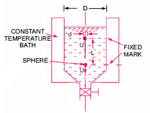


The force acting on the sphere are-
1) Weight W, acting vertically downward.
2) Buoyant force FB, acting vertically upward
3) Drag force FD, acting vertically upward.
W= volume × Density of sphere × g

FB = weight of liquid displaced
= volume of liquid displaced × density of liquid × g


For equilibrium


Rotating cylinder method:
In this method, Newton’s law of viscosity is used to measure the viscosity of a fluid.
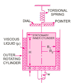
It consists of two concentric cylinders, the annular space between them is filled with the liquid whose viscosity is to be determined. The outer cylinder is rotated at a constant angular velocity with respect to the inner stationary cylinder. The torque transmitted by the enclosed liquid to the stationary cylinder is measured by the torsional strain of the restraining spring attached to the top of the inner cylinder.
According to Newton’s law of viscosity,

Since the annular space t = (R2 – R1) is quite small (where R2 and R1 are the radii of the outer and inner cylinders respectively), the velocity gradient

(Where N= the rotational speed of the outer cylinder in rpm)


(Where h = height of liquid)
Viscous torque = Viscous drag x radius

Viscous torque must be equal to the torque T exerted by the torquemeter.


Key Takeaway:


The velocity of the liquid layer adjacent to the pipe wall is zero when a liquid flows through a pipe. Due to viscosity, the velocity of the liquid increases as it approaches the wall, causing a velocity gradient and hence shear forces throughout the liquid. This viscous movement results in energy loss, which is commonly referred to as frictional loss.
William Froude developed the following fluid fraction laws for turbulent flow based on his experiments.
The frictional resistance for turbulent flow is :
- Proportional to
 where n fluctuates between 1.5 and 2.0
 - Proportional to fluid density
- Proportional to the area of the surface in contact
- Independent of pressure
- Dependant on the type of the surface in touch
Expression for Loss of Head Due to Friction in Pipes:
Consider a uniform horizontal pipe, having steady flow
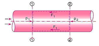


Applying Bernoulli's equations between sections 1-1 and 2-2,
Total head at 1-1 = Total head at 2-2 + loss of head due to friction between 1-1 and 2-2.


But  is the head lost due to friction and hence intensity of pressure will be reduced in the direction of flow by frictional resistance
Now,


The forces acting on the fluid between sections 1-1 and 2-2 are


Resolving all forces in the horizontal direction, we have


But,

So,


Putting,


This is known as Darchy-Weish-Bach Equation


Key Takeaway:

In a fully developed turbulent pipe flow, the friction factor is determined by the Reynolds number and relative roughness  , which is the ratio of the pipe's mean height of roughness to its diameter. All published results are acquired from tedious experiments employing intentionally roughened surfaces (typically by gluing sand grains of a given size on the inner surfaces of the pipes), and the functional form of this dependence cannot be obtained from a theoretical study.
The friction factor was determined using the flow rate and pressure drop readings.
Curve-fitting experimental data yielded tabular, graphical, and functional results, which are presented in tabular, graphical, and functional formats.
The Colebrook equation was created when Cyril.F. Colebrook (1910–1997) integrated the existing data for transition and turbulent flow in smooth and rough pipes into the following implicit relation.

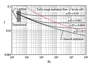
Lewis F. Moody (1880–1953) redrew Rouse's diagram into the current format two years later. It is given the now-famous Moody chart. It plots the Darcy friction factor for pipe flow as a function of Reynolds number and e/D over a wide range of Reynolds numbers and  values. It is one of the most extensively accepted and utilised engineering diagrams. Although it was designed for circular pipes, it can be used for noncircular pipes by substituting the hydraulic diameter for the diameter.
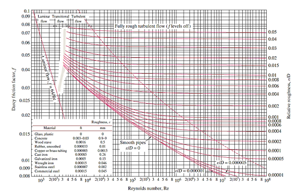
Commercially available pipes differ from those used in the trials in that their roughness is not uniform, making it impossible to give an exact description. Table and the Moody chart both show equivalent roughness levels for several commercial pipes.
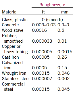
However, keep in mind that these figures are for fresh pipes, and as a result of corrosion, scale building, and precipitation, the relative roughness of pipes can rise over time. As a result, the friction factor could rise by 5 to 10 times. The design of piping systems must take into account actual operating circumstances. Furthermore, the Moody chart and its equivalent Colebrook equation are subject to a number of uncertainties (roughness size, experimental error, data curve fitting, and so on), therefore the findings produced should not be considered "precise." It's usually thought to be accurate to within  percent of the figure's range.
Because the Colebrook equation is implicit in f, iteration is required to determine the friction factor unless an equation solver such as EES is utilised. S. E. Haaland published an approximate explicit relation for f in 1983.

The findings derived from this relationship are within 2% of the Colebrook equation's results. When using a programmable calculator or a spreadsheet to solve for f with the equation, can be utilised as a good first guess in a Newton iteration if more exact results are required.
We make the following observations from the Moody chart:
- The friction factor for laminar flow decreases with rising Reynolds number and is unaffected by surface roughness.
- For a smooth pipe, the friction factor is lowest (although not zero because of the no-slip condition) and increases with roughness.In this scenario, the Colebrook equation
 reduces to the Prandtl equation.

- The shaded area in the Moody chart indicates the transition region from the laminar to turbulent regime (2300 < Re < 4000). Depending on flow disturbances, the flow in this region may be laminar or turbulent, or it may alternate between laminar and turbulent, causing the friction factor to fluctuate between values for laminar and turbulent flow. The information in this range is the least trustworthy. The friction factor increases in the transition area with modest relative roughness’s and approaches the value for smooth pipes.
- The friction factor curves corresponding to specified relative roughness curves are almost horizontal at very large Reynolds numbers (to the right of the dashed line in the chart), and hence the friction factors are independent of the Reynolds number. Because the thickness of the viscous sublayer drops with rising Reynolds number, it gets so thin that it is negligible in comparison to the surface roughness height, the flow in that region is referred to as fully rough, turbulent flow or simply fully rough flow. In this situation, the protruding roughness elements cause the viscous effects in the main flow, while the contribution of the laminar sublayer is insignificant.
- In the fully rough zone, the Colebrook equation reduces to the von Kármán equation stated as, which is clear in f. Although some publications refer to this zone as having wholly (or completely) turbulent flow, this is misleading because the flow to the left of the dashed blue line is likewise completely turbulent.

Key Takeaway:


Turbulent Shear Stress:
Consider turbulent flow in a horizontal pipe, and the upward eddy migration of fluid particles from a lower velocity layer to a higher velocity layer via a differential area  because of velocity fluctuations
  .
.
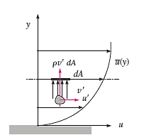
The overall effect of the mass flow rate of the fluid particles rising through  on the layer above dA is a reduction in its average flow velocity due to momentum transfer to the fluid particles with lower average flow velocity. This momentum transfer causes the fluid particles' horizontal velocity to increase by
  , and thus their momentum in the horizontal direction to grow at a rate of
  , which must be equal to the decrease in the higher fluid layer's momentum.
Given that the horizontal force acting on a fluid element above dA owing to the passage of fluid particles through dA is equal to the rate of change of momentum in that direction, the horizontal force acting on a fluid element above dA due to the passage of fluid particles through dA is,

Therefore, the shear force per unit area due to the eddy motion
Of fluid particles

Can be viewed as the instantaneous turbulent shear stress. Then the turbulent shear stress can be expressed as,

 is the time average of the product of the fluctuating velocity components
  &
& 

The results of experiments reveal that  is frequently a negative number. Terms such as
  or
or  are called Reynolds stresses or turbulent stresses.
In order to offer mathematical closure to the equations of motion, many semi-empirical formulations have been created that represent the Reynolds stress in terms of average velocity gradients. Turbulence models are examples of such models.
The random eddy motion of groups of particles is similar to the random motion of molecules in a gas, with molecules colliding after a set distance and transferring momentum in the process. As a result, momentum transport in turbulent flows via eddies is akin to molecular momentum diffusion. The turbulent shear stress is expressed in an analogous manner in many of the simpler turbulence models, as suggested by the French mathematician Joseph Boussinesq.

The eddy viscosity , also known as turbulent viscosity, accounts for momentum conveyance by turbulent eddies. The overall shear stress can then be readily represented as

Where,

The kinematic eddy viscosity or kinematic turbulent viscosity is denoted by the letter  . (also called the eddy diffusivity of momentum). Although the concept of eddy viscosity is intriguing, it is useless until its value can be established. Eddy viscosity must be represented as a function of the average flow variables, which is referred to as eddy viscosity closure. L. Prandtl introduced the concept of mixing length
  .
.

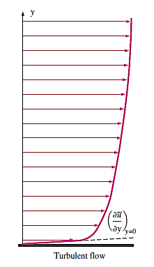
However, because lm is not a constant for a given flow, this concept is limited in application (in the vicinity of the wall). In the core region of a turbulent boundary layer, eddy motion and consequently eddy diffusivities are substantially bigger than their molecular equivalents. Because of the no-slip condition, the eddy motion loses its intensity near the wall and lessens at the wall. As a result, the velocity profile of a turbulent boundary layer changes slowly in the core but quickly in the thin layer near to the wall, resulting in substantial velocity gradients at the wall surface. It's no surprise, then, that the wall shear stress in turbulent flow is substantially higher than in laminar flow.
It's worth noting that molecular momentum diffusivity is a fluid attribute. Eddy diffusivity, on the other hand, is a flow attribute whose value is dependent on flow conditions. Eddy diffusivity reduces as you go closer to the wall, eventually reaching zero. Its value varies from zero at the wall to thousands of times the molecular diffusivity value in the core region.
Turbulent Velocity Profile:
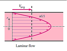
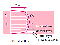
In contrast to laminar flow, the velocity profile expressions in turbulent flow are based on both analysis and observations, making them semi-empirical in nature with constants obtained from experimental data. Consider a pipe with fully developed turbulent flow, and let u denote the time averaged velocity in the axial direction (and remove the overbar from  for simplicity).
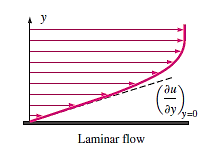
In laminar flow, the velocity profile is parabolic, but in turbulent flow, it is much fuller, with a dramatic decrease near the pipe wall. Turbulent flow over a wall can be divided into four areas, each of which is defined by its distance from the wall. The viscous (or laminar, linear, or wall) sublayer is a very thin layer adjacent to the wall where viscous effects are prevalent. This layer's velocity profile is virtually linear, and the flow is streamlined. Next to the viscous sublayer is the buffer layer, where turbulent effects are becoming more prominent but viscous effects still dominate the flow.
The overlap (or transition) layer, also known as the inertial sublayer, is above the buffer layer, where turbulence effects are significantly more prominent but still not dominant. Above that is the outer (or turbulent) layer, which dominates turbulent effects over molecular diffusion (viscous) effects in the remaining section of the flow.
Because flow properties vary greatly between regions, it's difficult to develop an analytic relationship for the velocity profile of the entire flow, as we did for laminar flow. In the turbulent situation, it turns out that utilising dimensional analysis to identify the essential variables and functional forms, and then using experimental data to estimate the numerical values of any constants, is the optimum technique.
The viscous sublayer has a very tiny thickness (usually less than 1% of the pipe diameter), yet due to the high velocity gradients it involves, this thin layer close to the wall has a significant impact on flow characteristics. Because the wall dampens any eddy motion, the flow in this layer is nearly laminar, and the shear stress is proportional to the fluid viscosity.
We would expect the velocity profile in this layer to be very nearly linear, given that velocity changes from zero to almost the core region value across a layer that is sometimes no thicker than a hair (almost like a step function).
Then the velocity gradient in the viscous sublayer remains nearly constant at

The wall shear stress


Were,


So,

This equation is known as the law of the wall,

Thickness of viscous sublayer,


The average velocity of a pipe is directly related to the flow velocity. As a result, we find that the viscous sublayer thickness is proportional to kinematic viscosity and inversely proportional to average flow velocity. In other words, when the velocity (and consequently the Reynolds number) rises, the viscous sublayer is suppressed, and it becomes thinner. As a result, at very high Reynolds numbers, the velocity profile becomes virtually flat, and the velocity distribution becomes more uniform.

The distance y from the surface is nondimensionalized using viscous length. It is easier to work with nondimensionalized distance and nondimensionalized velocity defined as in boundary layer analysis.
Nondimensionalized variables,


Then the law of the wall

When plotted against the logarithm of distance from the wall, the experimental data for velocity line up on a straight line in the overlap layer. The velocity in the overlap layer is proportional to the logarithm of distance, according to dimensional analysis and tests, and the velocity profile can be expressed.
The logarithmic law,


So,


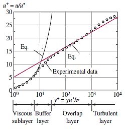


So,


The normalised velocity profile in the core region of turbulent flow in a pipe is dependent on the distance from the centreline and is independent of the fluid viscosity, as shown by this relationship. This is not surprising given that eddy motion dominates in this region and fluid viscosity has no effect.
Numerous other empirical velocity profiles exist for turbulent pipe flow. Among those, the simplest and the best known is the power-law velocity profile expressed as,


Where the exponent n is a constant whose value depends on the Reynolds number. The value of n increases with increasing Reynolds number. The value n = 7 generally approximates many flows in practice, giving rise to the term one-seventh power-law velocity profile.
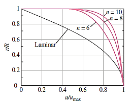
The turbulent velocity profile is fuller than the laminar one, and as n (and hence the Reynolds number) grows, it becomes more flat. It's also worth noting that the power-law profile can't be utilised to calculate wall shear stress because it gives an infinite velocity gradient and doesn't give a zero slope at the centreline. However, these discrepancies only account for a small percentage of the flow, and the power-law profile produces extremely accurate results for turbulent flow through a pipe.
Despite the viscous sublayer's thin thickness (often less than 1% of pipe diameter), the features of the flow in this layer are critical because they set the stage for flow in the rest of the pipe. Any imperfection or roughness on the surface disrupts this layer, causing the flow to be disrupted. As a result, unlike laminar flow, turbulent flow's friction factor is a strong function of surface roughness.
Key Takeaway:


Examples
Q.1. A pipeline carrying water has average height of irregularities projecting from the surface of the boundary of the pipe as 0.12 mm. What type of boundary is it? The shear stress developed is 4.9 N/m2. The kinematic viscosity of water is 0.01 strokes.
Solution:
Height of irregularities k= 0.15 mm

Shear stress 
Kinematic viscosity 
Density of water 
Step 1 Shear stress

Step 2 Roughness Reynolds’s number

Since Re > 4 but less than 100 the surface is transition
Q.2. For turbulent flow through a pipe having wall shear stress 10 N/m², size of surface imperfection is k = 0.03 mm. Assuming the kinematic viscosity of water 1 x 10 m³/sec. Find whether pipe behave as hydro dynamically rough, smooth or transitional.
Solution:
Shear stress  = 10 N/m²
Size of surface imperfection k= 0.03 mm = 0.03 x 10³ m
Kinematic viscosity v = 1x10 m²/sec.
Density of water  = 1000 kg/m³
Step 1: Shear stress,

Step 2: Roughness Reynolds’s number,

Re= 0.03 < 4
Since  less than 4, between 4 and 100, and hence pipe Since surface behaves as smooth.
Q.3. A pipe line carrying oil s= 0.8 has average height of irregularities projecting from the surface of the boundary of the pipe as 0.3 mm. What type of boundary is it? The shear stress developed is 3N/m². Take kinematic viscosity v = 0,012 stoke.
Solution:
Average height of irregularities K = 0.3 mm = 0.3 x 10³ m
Shear stress =3 N/mm²
Specific gravity of oil s=0.8.
Density p=800 kg-m¹
Kinematic viscosity v=0.012 stoke=0.012x 10 m²/sec.
Step 1: Shear stress,

Step 2: Roughness Reynolds’s number,

15.25> 4 but <100
The surface boundary is transition.
Q.4. Air (p = 1.22 kg/m³ and v = 1.5 x 10 m³/s) flows through 250 mm diameter pipe at 8 m/s as mean velocity. If the equivalent sand grain roughness is 0.5 mm, calculate wall shear stress and friction factor f. Assume flow to be fully rough, turbulent and neglect compressibility.
Solution:
p = 1.22 kg/m²
v = 1.5x 10³ m²/sec.
d = 250 mm = 0.25 m.
R= 0.125 m, u = 8 m/sec.,
K = 0.5 mm = 5 x 10¹ m
Step 1: Reynolds’s number

The flow is turbulent in the rough pipe.
Step 2: For rough turbulent pipe

Step 3: Shear stress at the pipe surface

The wall shear stress is 0.134 N/m² and friction factor is 0.0137.
Q.5. Determine the wall shearing stress in a pipe of diameter 100 mm which carries water. The velocities at the pipe centre and 30 mm from the pipe centre are 2 m/s and 1.5 m/s respectively. The flow in pipe is given as turbulent.
Solution:
Diameter, D = 100 mm = 0.1 m,
Radius, R = 50 mm = 0.05 m
Velocity of centre, U = 2 m/sec
Velocity of 30 mm from centre u = 1.5 m/s,
y = 0.05-0.03 = 0.02 m
For turbulent flow,


Wall shear stress,


Q.6. In a pipe of diameter 150 mm, carrying water the velocities at the pipe centre and 45 mm from pipe centre are found to be 2.5 m/s and 2 m/s respectively. Find the wall shearing stress.
Solution:
Diameter of pipe D = 150 mm = 0.15m,
Radius R = 0.15/2 = 0.075 m 2
Velocity of centre U=2.5 m/s,
Velocity at 45mm
U = 2 m/sec
At u = 2 m/sec, y = 0.075 -0.045 = 0.03 m
For turbulent Velocity


Shear stress,


Q.7. In a pipe of diameter 100 mm carrying water, the velocities at the pipe centre and 20 mm from the pipe centre are found to be 2.5 ms and 2.3 m/s respectively. Find the wall shear stress.
Solution:
D-100 mm-0.1m,
Radius R=005 m.
Velocity at centre U=2.5 m/s,
Velocity at 20 mm
u=2.3 m/s,
Velocity 2.3 m/s from pipe wall, y=0.05-0.02 -0.03m
For Turbulent flow


Shear stress


Q.8. In a smooth pipe of diameter 0.5 m and length 900 m, water is flowing at a rate of 0.05 m/sec. Assuming kinematic viscosity of water as 0.02 stokes, find:
(1) Head lost due to friction
(2) Centre line velocity sub layer.
(3) Wall shear stress
(4) Thickness of laminar
Take friction factor f= 0.314/(Re)^(1/4) for turbulent.
Solution:
d=0.5 m.
L=900 m. Q=0.05 m/sec.
V= 0.02 stokes.
Step 1: Mean velocity,

Step 2: Reynolds’s number,

Step 3: The flow is turbulent,

Step 4: Head loss by Darcy-Weisbach equation,

Step 5: Wall shear stress,

Step 6: Shear velocity.

Step 7: For turbulent flow in smooth pipe, maximum velocity is,

For y=-=0.25 m, v = (1.e. Centre line viscosity)

Step 8: Thickness of laminar sub-layer

Q.9. Two Pitot-Prandtl tubes are used to find the velocities at the middle and the quarter point of a circular pipe simultaneously. Find the discharge of water (Assuming turbulent flow)if the diameter of the pipe is 300 mm and readings of the tubes are 2.53 m/s and 2.29 m/s.
Solution:
Diameter d = 300 mm = 0.3 m.
Velocity at middle u max=2.53 m/s at y = 0 Velocity at quarter Point of a circular pipe u = 2.29 m/s at y = 0.075
Step 1: Now for turbulent flow,


At y = 0.075

 …(Eq.1)
Step 2: At y=0 u. = 3.75,


Put u* in equation 1


Step 3: Discharge.


Q.10. For turbulent flow in circular pipe of radius 'r friction factor is 0.02 Estimate the local velocity at a radial distance 0.25 r from the axis of the pipe. If mean velocity is 0.3 m/s, what will be the velocity at the centre line of pipe?
Solution:
Radius R = r,
Frictional factor f=0.02,
Radial distance 10.25 r
Mean velocity u 0.3 m/s
Step 1: By Karman-Prandtl resistance equation for rough pipe is,


Step 2: Now using equation,


Step 3: Now for smooth and rough pipes,


Step 4: Maximum velocity occurs at centre-line of pipe, r = 0, u = u max


Local velocity at 0.25 r from axis of pipe is 0.3455 m /s and velocity at centre line is 0.356 m/sec.
Q.11. Determine the head loss in kPa for a pipe line 700 m long carrying petrol at the flow rate of 200 Lps. (p = 730 kg/m³, μ = 2.92 x 10 N-s/m²). The diameter of the pipe is 30 cm and the equivalent roughness magnitude is 0.3 mm. Use Moody's diagram.
Solution:
L = 700 m long,
Q = 200 Lps= 0.2 m³/sec,
p = 730 kg/m³, μ = 2.92 x 10 N-s/m².
d = 30 cm = 0.3 m, e = 0.3 mm = 0.3 x 10³ m
Step 1: Velocity,

Step 2: Relative roughness,

Step 3: Reynolds’s number,

Step 4: Refer Moody's diagram and R., we get

Step 5: Head loss by Darcy's equation,

Step 6: Head loss in kPa (pressure),

= 132.98 x 10³ mPa
p = 132.98 kPa
:. The head loss in kPa is 132.98 kPa.
Q.12. Determine the head lost in a diameter 300 m, 300 m long cast iron pipe when (1) Water at 15°C flow at a velocity 15 nvs and (ii) Fuel oil at 15°C flow at the same velocity. Assume size of surface imperfection 0.244 mm. Refer Moody's diagram. Take the following properties.
Fluid | Density (kg/m^3 ) | Viscosity (m^2/s) |
Water | 999.1 | 1.141x10^-6 |
Fuel oil | 858 | 4.41x10^-6 |
Solution:
L = 300 m, d = 300 mm = 0.3 m,
c = 0.244, V = 15 m/sec.
Case I: When water is flow with velocity = 15 m/sec.
e = 0.244
Step 1: Relative roughness

Step 2: Reynolds number


Step 3: Use moody's table for R. And values,
f = 0.0186
Step 4: Head loss by Darcy's equation,

Case II: When oil flows with same velocity 1.5 m/sec,

:. By using Moody's curve for Re and e/d values,
f = 0.0215
Head loss

References:
- Fluid Mechanics and Hydraulic Machines by R.K. Bansal, Laxmi Publications
- Fluid Mechanics: Fundamentals and Applications by Y. A. Çengel and J. M. Cimbala, by McGraw-Hill
- Fluid Mechanics by Frank .M. White, mcgraw Hill Publishing Company Ltd.
- Fundamentals of Fluid Mechanics by munson, Wiley India Pvt. Ltd