UNIT – V
Differentiation of functions of single variable
5.1 Differentiation of functions of single variable (excluding trigonometric functions)
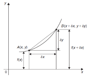
Differentiation from first principal-
A and B are the two point on a curve representing small increment in the x and y directions respectively. Gradient of chord-
However-
Hence-
Here When determining the gradient of a tangent to a curve there are two notations used. The gradient of the curve at A can either be written as,
Where
Or we can write it as-
Example: Differentiate the function f(x) = Sol. We know that-
Here
Substituting (
Hence-
|
Differentiation of common functions-
f(x) | dy/dx |
|
|
Sin ax | a cos ax |
Cos ax | -a sin ax |
|
|
Log ax | 1/x |
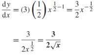
Example: Find the derivative of y = 3 Sol. We can write the given function y = 3 y = 3 so that-
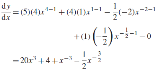
Example: Differentiate with respect to x-
Sol. The given function can be written in the form
Now-
Differentiation of a product- When y = uv and u, v are both function of x- then
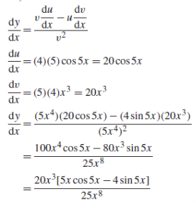
Differentiation of a quitient- When y = u/v and u,v are the functions of x- Then-
Example: Differential the following function-
Sol. We know that-
|
Key takeaways-
5.2 Break-even analysis
Meaning of Break-even-analysis:
The study of cost-volume profit analysis is often referred to as ‘break-even analysis’ and the two terms are used interchangeably by many. This is so, because break-even analysis is the most widely known form of cost-volume-profit analysis. The term “break-even analysis” is used in two senses—narrow sense and broad sense.
In its broad sense, break-even analysis refers to the study of relationship between costs, volume and” profit at different levels of sales or production. In its narrow sense, it refers to a technique of determining that level of operations where total revenues equal total expenses, i.e., the point of no profit, no loss.
Break-even-point:
The break-even point is the level of production n where the revenue from the sales is equal to the cost of production n. At the break vent point, the company is neither making a profit nor losing money.
Consumption Function. If/ denotes the total national income and C denotes the total national consumption, then the function
C = f(l)
relating/ and C is called the consumption function. The difference between / and consumption C is savings S. Thus S • I - C.
Question 1: A house finds that the cost of product ion directly attributed to each book is Rs.40 and that the fixed costs are Rs. 25,000. If each book can be sold for R. s 60, then
{i) the cost function,
(ii) the revenue function,
the profit function, and
the break-even point.
Sol (1) Let number of books published by the publishing house is x.
Variable cost = 40x and fixed cost = Rs. 25, 000
Hence the total cost function, C (x), may be written as
C (x) = 40x + 25000
(ii,) Since the book is sold for Rs. 60, the revenue function, R is given by (x)
R (x) = 60
Profit function, P (x), is given by
P (x) = R(x) - C (x) = 60x - 40x - 25000 = 20x - 25000.
At the break-even point, P (x) = 0. That is,
20x - 25000 = 0 i.e., x = 1250
Hence 1250 books should be produced and sold to achieve break-even point.
2. Consider the following data of a company:
Sales = Rs. 40,000;
Fixed cost = Rs. 7500;
Variable cost = Rs. 17,500;
Find the following: (a) Contribution (b) Profit (c) BEP (d) M.S.
Given Data:
Sales = Rs. 40,000
Fixed cost = Rs. 7,500
Total variable cost = Rs.17,500
Formula Used:
Contribution = Sales – Total variable costs
Profit = Contribution - Fixed cost
BEP = Fixed cost / (P/V ratio)
P/V ratio = Contribution / sales
M.S. = Profit / (P/V ratio)
Solution:
(a) Contribution = Sales – Total variable costs
= Rs. 40,000 - Rs. 17,500
= Rs. 22,500
(b) Profit = Contribution - Fixed cost
= Rs. 22,500 - Rs. 7,500
= Rs. 15,000
(c) BEP = Fixed cost / (P/V ratio)
P/V ratio = Contribution / sales
= 22,500 / 40,000
= 0.5625
P/V ratio in percent = 0.5625 x 100 = 56.25%
BEP = 7,500 / 0.5625
= Rs. 13,333.33
(d) M.S. = Profit / (P/V ratio)
= 15,000 / 0.5625
= Rs. 26,666.67
Key Takeaways:
- Break-even analysis refers to the study of relationship between costs, volume and” profit at different levels of sales or production.
- In its narrow sense, it refers to a technique of determining that level of operations where total revenues equal total expenses, i.e., the point of no profit, no loss.
- The break-even point is the level of production n where the revenue from the sales is equal to the cost of production n. At the break vent point, the company is neither making a profit nor losing money.
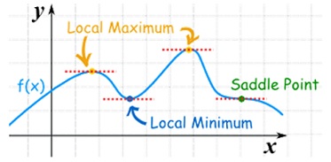
A function f(x) is said to be maximum at x = a if f(a) is greater than every other value of f(x) in the immediate neighbourhood of x = a (i.e., f(x) ceases to increase but begins to increase at x = a. Similarly the minimum
value of f(x) will be that value at x = b which is less than other values in the immediate neighbourhood of x= b.
Maxima and minima of function of two variables-
As we know that the value of a function at maximum
Point is called maximum value of a function. Similarly the value of a function at minimum point is called minimum value of a function.
The maxima and minima of a function is an extreme biggest and extreme smallest point of a function in a given range (interval) or entire region. Pierre de Fermat was the first mathematician to discover general method for calculating maxima and minima of a function. The maxima and minima are complement of each other.
Maxima and Minima of a function of one variables
If f(x) is a single valued function defined in a region R then
Maxima is a maximum point  if and only if
Minima is a minimum point  if and only if
|


Maxima and Minima of a function of two independent variables
Let  be a defined function of two independent variables.
Then the point  is said to be a maximum point of
  if
if

Or  =
= 
For all positive and negative values of h and k.
Similarly the point  is said to be a minimum point of
  if
if

Or  =
= 
For all positive and negative values of h and k.
Saddle point: Critical points of a function of two variables are those points at which both partial derivatives of the function are zero. A critical point of a function of a single variable is either a local maximum, a local minimum, or neither. With functions of two variables there is a fourth possibility - a saddle point.
Note-
- Maximum and minimum values of a function occur alternatively
- Function may have several maximum and minimum values in an interval
- At some point the maximum value may be less than the minimum value
- The points at which a function has maximum or minimum value are called turning points and the maximum and minimum values are known as extreme values, or extremum or turning values.
- The values of x for which f(x) = 0 are often called critical values
Criteria for maximum and minimum-
For a function y = f(x) to attain a maximum point at x = a,

For minimum point-

Conditions for max. and min-
Necessary Condition- If a function f(x) is maximum or minimum at a point x = b and if f’(b) exists then f’ (b) = 0.
Sufficient Condition-If b is a point in an interval where f(x) is defined and if f ‘(b) = 0 and f’’(b)  0, then f(b) is maximum if f’’(b) <0 and is minimum if f’’(b) > 0. (The proof is not shown at present).
Working Rule:
First derivative method
To find the maximum or minimum point of a curve y = f(x).
Find f ‘(x) and equate it to zero. From the equation f ‘(x) = 0, find the value of x, say a and b.
Here the number of roots of f ‘(x) = 0 will be equal to the number of degree of f ‘(x) = 0.
Then find f ‘(a – h) and f ‘(a + h), then note the change of sign if any (here h is very small).
If the change is from positive to negative, f(x) will be maximum at x = a. If again the change of sign is from negative to positive, f(x) will be maximum at x = a.
Similarly for x = b.
Second derivative method-
First, we find the first derivative of y = f(x) i.e., dy/dx and make it zero.
From the equation  find the value of x say a and b.
The again we find the second derivative of y or  .
.
Put x = a in  , if
, if  at x = a is negative then the function is maximum at x = a and maximum value will be f(a).
If the value of  at x = a is positive, then the function is minimum and the minimum value will be f(a)
Similarly we take for x = b.
Example: Examine for maximum and minimum for the function f(x) = Sol. Here the first derivative is-
So that, we get-
Now we will get to know that the function is maximum or minimum at these values of x. For x = 3 Let us assign to x, the values of 3 – h and 3 + h (here h is very small) and put these values at f(x). Then-
Thus f’(x) changes sign from negative to positive as it passes through x = 3. So that f(x) is minimum at x = 3 and the minimum value is-
And f(x) is maximum at x = -3.
Example: Find out the value of x for which the function f(x) = Sol. Let y = f(x) = Then the first derivative will be-
Putting
By using middle term splitting- We get-
Now we will find the second derivative- We get-
Here At x = 4, At x = 16,
|
Key takeaways-
- The value of a function at maximum point is called maximum value of a function. Similarly the value of a function at minimum point is called minimum value of a function.
- For a function y = f(x) to attain a maximum point at x = a,

For minimum point-

3. Necessary Condition- If a function f(x) is maximum or minimum at a point x = b and if f’(b) exists then f’ (b) = 0.
Sufficient Condition- If b is a point in an interval where f(x) is defined and if f ‘(b) = 0 and f’’(b)  0, then f(b) is maximum if f’’(b) <0 and is minimum if f’’(b) > 0. (The proof is not shown at present).
References
- Mathematics and Statistics for Business – R. S. Bhardwaj – Excel Books.
- Business Mathematics and Statistics – Subhanjali Chopra – Pearson publication.
- Fundamentals of Business Mathematics and Statistics – ICAI – ICAI.
- Business Mathematics and Statistics – Dr. J K Das, N Das – McGraw Hill Education.
