Unit 5

Complex Number

5.1 Circular functions

In probability theory and statistics, complex random variables are a generalization of real-valued random variables to complex numbers, i.e. the possible values a complex random variable may take are complex numbers.[1] Complex random variables can always be considered as pairs of real random variables: their real and imaginary parts. Therefore, the distribution of one complex random variable may be interpreted as the joint distribution of two real random variables.

Some concepts of real random variables have a straightforward generalization to complex random variables—e.g., the definition of the mean of a complex random variable. Other concepts are unique to complex random variables.

            * A complex random variable ZZ {\displaystyle Z}  on the probability space ( Ω , F , P ) {\displaystyle (\Omega ,{\mathcal {F}},P)}(is a function Z : Ω → C {\displaystyle Z\colon \Omega \rightarrow \mathbb {C} }  on Z: ,such that both its real part ℜ ( Z ) {\displaystyle \Re {(Z)}} R(z) and its imaginary part i(z) ℑ ( Z ) {\displaystyle \Im {(Z)}} are real random variables on ( Ω , F , P ) {\displaystyle (\Omega ,{\mathcal {F}},P)}..

Circular symmetric complex normal random variables are used extensively in signal processing, and are sometimes referred to as just complex normal in signal processing literature.  Formally, is a standard complex normal random variable.

The characteristic function of complex normal distribution is given by is a n -dimensional complex vector. Central limit theorem. If. The modulus of a complex normal random variable follows a Hoyt distribution

Example:1 Find fourth root of

Solution: Convert to polar first:  r=

Example:2 Find the fifth root of 4-4i of

Solution: Convert 4-4i to polar: r==;()cis()

5.2 Hyperbolic and Inverse Hyperbolic functions

Example1: Solve cosh2 x – sinh2 x

Solution:

Given: cosh2 x – sinh2 x

We know that

Sinh x = [ex– e-x]/2

Cosh x = [ex + e-x]/2

Cosh2 x – sinh2 x = [ [ex + e-x]/2 ]2 – [ [ex – e-x]/2 ]2

Cosh2 x – sinh2 x = (4ex-x) /4

Cosh2 x – sinh2 x = (4e0) /4

Cosh2 x – sinh2 x = 4(1) /4 = 1

Therefore, cosh2 x – sinh2 x = 1

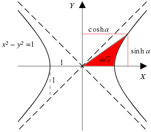
A ray through the unit hyperbola x 2   −   y 2   =   1 {\displaystyle \scriptstyle x^{2}\ -\ y^{2}\ =\ 1} in the point ( cosh a , sinh a ) {\displaystyle \scriptstyle (\cosh \,a,\,\sinh \,a)} , where a {\displaystyle \scriptstyle a} is twice the area between the ray, the hyperbola, and the x {\displaystyle \scriptstyle x} -axis

Example 2:

Find the inverse of the function f(x) = ln(x – 2)

Solution:

First, replace f(x) with y

So, y = ln(x – 2)

Replace the equation in exponential way , x – 2 = ey

Now, solving for x,

x = 2 + ey

Now, replace x with y and thus, f-1(x) = y = 2 + ey

Example 3:

To solve an equation: f(x) = 2x + 3, at x = 4

Solution:

We have,

f(4) = 2 × 4 + 3

f(4) = 11

Now, let’s apply for reverse on 11.

f-1(11) = (11 – 3) / 2

f-1(11) = 4

Magically we get 4 again.

Therefore, f(f(4)) = f(4)

So, when we apply function f and its reverse f-1 gives the original value back again, i.e, f-1(f(x)) = x.

5.3 Logarithms of a complex number

Example1:  Prove that function is analytic function.

Solution. Real and Imaginary parts of are

If,

On differentiating u,v we get

Again differentiating

Example2: Determine P such that the function analytic

Solution:     

Hence  

f(z) is analytic Cauchy Riemann should be satisfied that is

And                            

P=-1

5.4 Resolving real and imaginary parts of a complex number.

Example 1:

Problem: simplify 16 i+10i (3-i)

Solution:

Given,

16i +10i (3-i)

=16i+10i (3i) +10 i(-i)

=16i+30i-10i2

=46i-10(-1)

=46i+10

Here real part is 10 and imaginary part is 46

Example 2:

Problem: express the following into a+ib form

Solution:

Given.,     

z   =        = = + i

Modulus , =   = = 

Conjugate = (  - 

Reference Book:

1. G.B. Thomas and R.L. Finney, Calculus and Analytic geometry, 9th Edition, Pearson, Reprint, 2002.

2. Erwin kreyszig, Advanced Engineering Mathematics, 9th Edition, John Wiley & Sons,2006.

3. Veerarajan T., Engineering Mathematics for the first year, Tata McGraw-Hill, New Delhi,2008.

4. Ramana B.V., Higher Engineering Mathematics, Tata McGraw Hill New Delhi, 11th Reprint, 2010.

5. D. Poole, Linear Algebra: A Modern Introduction, 2nd Edition, Brooks/Cole, 2005.

6. B.S. Grewal, Higher Engineering Mathematics, Khanna Publishers, 36th Edition, 2010