4.1 Solution of Ordinary differential equations by Taylor’s series and Picard’s method

Back to Study material

M-II

UNIT-4

Numerical methods

4.1 Solution of Ordinary differential equations: by Taylor’s series and Picard’s method

The general first order differential equation

…. (1)

With the initial condition …(2)

In general, the solution of first order differential equation in one of the two forms:

a) A series for y in terms of power of x, from which the value of y can be obtained by direct solution.

b) A set of tabulated values of x and y.

The case (a) is solved by Taylor’s Series or Picard method whereas case (b) is solved by Euler’s, Runge Kutta Methods etc.

Taylor’s Series Method:

The general first order differential equation

….(1)

With the initial condition …(2)

Let be the exact solution of equation (1), then the Taylor’s series for around is given by

(3)

If the values of are known, then equation (3) gives a power series for y. By total derivatives we have

And other higher derivatives of y. The method can easily be extended to simultaneous and higher –order differential equations. In general,

Putting in these above results, we can obtain the values of finally, we substitute these values of in equation (2) and obtain the approximate value of y; i.e. the solutions of (1).

Example1: Solve, using Taylor’s series method and compute .

Here This implies that .

Differentiating, we get

The Taylor’s series at ,

(1)

At in equation (1) we get

Example2: Using Taylor’s series method, find the solution of

At ?

Here

At implies that or or

Differentiating, we get

implies that or .

implies that or

The Taylor’s series at ,

(1)

At in equation (1) we get

Example3: Solve numerically, start from and carry to using Taylor’s series method.

Here .

We have

Differentiating, we get

implies that or

implies that or .

implies that

The Taylor’s series at ,

Here

The Taylor’s series

Picard’s method of successive approximation-

The P.I. of the initial value problem having an ODE-

With initial condition is obtained by integrating (1), then-

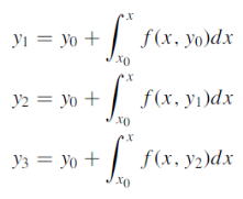
In the Picard’s method, the first approximation y1 is obtained by replacing y in f (x, y) in RHS of (2) by y0 and then evaluating the integral (which is now a function of x) w.r.t x. The second approximation y2 is then obtained by replacing y in f (x, y) of RHS of (2) by y1 and integrating w.r.t x. Successive approximations are obtained similarly. In practice, Picard’s method is restricted to a limited class of problems in which the integral in RHS of (2) can be evaluated.

So that-

…………………………..

…………………………….

Example: Obtain the Picard’s second approximation for the initial value problem-

Find y(1).

Sol.

The first approximation-

Replace y by , we get-

Replace y by , we get the second approximation-

Third approximation-

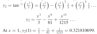
Here we find that the integration is very difficult.

Now expanding , from the second approximation-

We get-

4.2 Runge-Kutta method of fourth order for solving first order equations

This method is more accurate than Euler’s method.

Consider the differential equation of first order

Let be the first interval.

A second order Runge Kutta formula

Where

Rewrite as

A fourth order Runge Kutta formula:

Where

Example1: Use Runge Kutta method to find y when x=1.2 in step of h=0.1 given that

Given equation

Here

Also

By Runge Kutta formula for first interval

Again

A fourth order Runge Kutta formula:

To find y at

A fourth order Runge Kutta formula:

Example2: Apply Runge Kutta fourth order method to find an approximate value of y for x=0.2 in step of 0.1, if

Given equation

Here

Also

By Runge Kutta formula for first interval

A fourth order Runge Kutta formula:

Again

A fourth order Runge Kutta formula:

Example3: Using Runge Kutta method of fourth order, solve

Given equation

Here

Also

By Runge Kutta formula for first interval

)

A fourth order Runge Kutta formula:

Hence at x = 0.2 then y = 1.196

To find the value of y at x=0.4. In this case

A fourth order Runge Kutta formula:

Hence at x = 0.4 then y=1.37527

Solution of Second order ODE using 4th order Runge-Kutta method:

The second order differential equation

Let then the above equation reduces to first order simultaneous differential equation

Then

This can be solved as we discuss above by Runge Kutta Method. Here for and for .

A fourth order Runge Kutta formula:

Where

Example1: Using Runge Kutta method of order four , solve to find

Given second order differential equation is

Let then above equation reduces to

(say)

Or .

By Runge Kutta Method we have

A fourth order Runge Kutta formula:

Example2: Using Runge Kutta method, solve

for correct to four decimal places with initial condition .

Given second order differential equation is

Let then above equation reduces to

(say)

Or .

By Runge-Kutta Method we have

A fourth order Runge Kutta formula:

And

Example3: Solve the differential equations

for

Using four order Runge Kutta method with initial conditions

Given differential equation are

Let

And

Also

By Runge Kutta Method we have

A fourth order Runge Kutta formula:

And

4.3 Numerical integration: Trapezoidal rule and Simpson’s 1/3rd and 3/8 rules

Numerical integration is a process of evaluating or obtaining a definite integral from a set of numerical values of the integrand f(x).In case of function of single variable, the process is called quadrature.

Trapezoidal Method:

Let the interval [a, b] be divided into ‘n’ equal intervals such

that <<….<=b.

Here .

To find the value of .

Setting n=1, we get

I =

The above is known as Trapezoidal method.

Note: In this method second and higher difference are neglected and so f(x) is a polynomial of degree 1.

Geometrical Significance: The curve y=f(x), is replaced by n straight lines with the points ();() and ();…….;() and ().

The area bounded by the curve y=f(x), the ordinates ,and the x axis is approximately equivalent to the sum of the area of the n trapeziums obtained.

Example1: State the trapezoidal rule for finding an approximate area under the given curve. A curve is given by the points (x, y) given below:

(0, 23), (0.5, 19), (1.0, 14), (1.5, 11), (2.0, 12.5), (2.5, 16), (3.0, 19), (3.5, 20), (4.0, 20).

Estimate the area bounded by the curve, the x axis and the extreme ordinates.

We construct the data table:

X	0	0.5	1.0	1.5	2.0	2.5	3.0	3.5	4.0
Y	23	19	14	11	12.5	16	19	20	20

Here length of interval h =0.5, initial value a = 0 and final value b = 4

By Trapezoidal method

Area of curve bounded on x axis =

Example2: Compute the value of

Using the trapezoidal rule with h=0.5, 0.25 and 0.125.

Here

For h=0.5, we construct the data table:

X	0	0.5	1
Y	1	0.8	0.5

By Trapezoidal rule

For h=0.25, we construct the data table:

X	0	0.25	0.5	0.75	1
Y	1	0.94117	0.8	0.64	0.5

By Trapezoidal rule

For h = 0.125, we construct the data table:

X	0	0.125	0.25	0.375	0.5	0.625	0.75	0.875	1
Y	1	0.98461	0.94117	0.87671	0.8	0.71910	0.64	0.56637	0.5

By Trapezoidal rule

[(1+0.5)+2(0.98461+0.94117+0.87671+0.8+0.71910+0.64+0.56637)]

Example3: Evaluate, using trapezoidal rule with five ordinates

Here

We construct the data table:

X	0
Y	0	0.3693161	1.195328	1.7926992	1.477265	0

Simpson’s Rule:

Let the interval [a, b] be divided into ‘n’ equal intervals such that <<….<=b.

Here .

To find the value of .

Setting n = 2,

Which is known as Simpson’s 1/3- rule or Simpson’s rule.

Note: In this rule third and higher differences are neglected so f(x) is a polynomial of degree 2.

Example1: Estimate the value of the integral

by Simpson’s rule with 4 strips and 8 strips respectively

For n=4, we have

We construct the data table:

X	1.0	1.5	2.0	2.5	3.0
Y=1/x	1	0.66666	0.5	0.4	0.33333

By Simpson’s Rule

For n = 8, we have

X	1	1.25	1.50	1.75	2.0	2.25	2.50	2.75	3.0
Y=1/x	1	0.8	0.66666	0.571428	0.5	0.444444	0.4	0.3636363	0.333333

By Simpson’s Rule

Example2: Evaluate

Using Simpson’s 1/3 rule with .

For , we construct the data table:

X	0
	0	0.50874	0.707106	0.840896	0.930604	0.98281	1

By Simpson’s Rule

Example3:Using Simpson’s 1/3 rule with h = 1, evaluate

For h = 1, we construct the data table:

X	3	4	5	6	7
	9.88751	22.108709	40.23594	64.503340	95.34959

By Simpson’s Rule

= 177.3853

Simpson’s 3/8 rule

Let the interval [a, b] be divided into n equal intervals such that <<….<=b.

Here .

To find the value of .

Setting n=3 , we get

Is known as Simpson’s 3/8 rule which is not as accurate as Simpson’s rule.

Note: In this rule the fourth and higher differences are neglected and so f(x) is a polynomial of degree 3.

Example: Evaluate By Simpson’s 3/8 rule.

Let us divide the range of the interval [4, 5.2] into six equal parts.

For h=0.2, we construct the data table:

4.0

4.2

4.6

4.8

5.0

5.2

Y=logx

1.3863

1.4351

1.4816

1.5261

1.5686

1.6094

1.6487

By Simpson’s 3/8 rule

= 1.8278475

Example2: Evaluate

Let us divide the range of the interval [0,6] into six equal parts.

For h=1, we construct the data table:

X	0	1	2	3	4	5	6
	1	0.5	0.2	0.1	0.0588	0.0385	0.027

By Simpson’s 3/8 rule

+3(0.0385)+0.027]

=1.3571

Error in Integration-

Error in Trapezoidal method

The total error in trapezoidal method is given by

Let is the largest value of the n quantities on the right hand side of the above equation then

Error in Simpson’s Rule

The error in the Simpson’s rule is given by

Where is the largest value of the fourth derivative of y(x).

Error in Simpson’s 3/8 Rule

The error in this rule is given by

Where is the largest value of the derivative of y(x)

References

E. Kreyszig, “Advanced Engineering Mathematics”, John Wiley & Sons, 2006.
P. G. Hoel, S. C. Port And C. J. Stone, “Introduction To Probability Theory”, Universal Book Stall, 2003.
S. Ross, “A First Course in Probability”, Pearson Education India, 2002.
W. Feller, “An Introduction To Probability Theory and Its Applications”, Vol. 1, Wiley, 1968.
N.P. Bali and M. Goyal, “A Text Book of Engineering Mathematics”, Laxmi Publications, 2010.
B.S. Grewal, “Higher Engineering Mathematics”, Khanna Publishers, 2000.
T. Veerarajan, “Engineering Mathematics”, Tata Mcgraw-Hill, New Delhi, 2010
Higher engineering mathematics, HK Dass
BV ramana, higher engineering mathematics

Sign Up

Index

Notes

Highlighted

Underlined

Browse by Topics

Notes

Highlighted

Underlined