Unit 3
The households
Budget line
Knowledge of the concept of budget lines is important for understanding the idea of consumer equilibrium. The higher apathy curve shows higher satisfaction than the lower one. Therefore, the consumer in his attempt to maximize his satisfaction will try to reach the highest possible indifference curve.
However, in order to buy more goods and seek to get more satisfaction, he must work under two constraints; firstly, he must pay the price of the goods, and secondly, he has a limited money income to buy the goods. Therefore, how far he will go for his purchase depends on the price of the goods and the income of the money he will have to spend on the goods.
Now, in order to explain the equilibrium of consumers, it is also necessary to introduce into the indifferent diagram a budget line, which represents the price of goods and the income of consumers ' money.
Suppose that our consumers have Rs income. Let's say Rs the price of a good X in the market to spend on 50 goods X and Y. That of 10 and Y Rs per unit. 5 per unit if the consumer spends his entire income of Rs. In a good X 50,he would buy 5 units of X;if he spent his entire income of Rs. To 50 good Y he would buy 10 units of Y if a straight line connecting 5X and 10Y is drawn, we get what is called a price line or budget line.
This budget line looks at all the figures of two goods a consumer can buy by spending his given money income on two goods at a given price. 8.14 show it in Rs. The price of 50 and X and Y is Rs. 10 and Rs. 5 respectively consumers can buy 10Y and OX, or 8Y and IX;or 6Y and 2X, or 4Y and 3x etc.
In other words, he can buy any combination that is on the budget line at the given price of the goods with the income of his given money. It should be noted that the combination of goods as H (5Y and 4x) above and outside the given budget line is beyond the reach of consumers.
However, a combination that is within the budget line, such as k (2X and 2Y), is within the reach of die consumer, but buying such a combination will not spend all the proceeds of the Rs. 50. Therefore, on the assumption that the totality of the given income will be spent on the given goods and at the given price, the consumer must choose from all the combinations that are on the budget line. It is also clear that over budget lines give a graphical budget. The combination of goods to the right of the budget line is unattainable, since the consumer's income is not enough to be able to buy those combinations. Given his income and the price of goods, the combination of goods on the left side of the budget line is achievable, that is, the consumer can buy any of them.
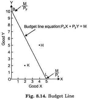
It is also important to remember that it is an intercept OB on the Y-axis in the figure. 8.14 is OB=M/Py, equal to the amount of his overall income divided by the price of goods Y. Similarly, The Intercept OL on the x-axis measures the total revenue divided by the price of the product X.OL=M / Vx. Where Px and Py represent the price of goods X and Irrespectively, and M represents the income of money. The above budget line formula (8.1) means that given the consumer's money income and the price of two goods, all the combinations lying on the budget line will cost the same amount and can therefore be purchased at a given income. A budget line can be defined as a set of a combination of two goods that can be purchased if the whole of a given income is spent on them and its slope is adequate to the negative of the worth ratio.
Budget space:
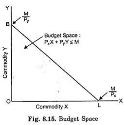
It is necessary to carefully understand that the budget equation PxX+PyY=M or Y=M/Py–Px/Py. X is indicated by the budget line in the figure. 8.14 only describe budget lines, not budget spaces. Budget space indicates a set of combinations of all goods that can be purchased by spending all or part of the given income. In other words, budget space represents all those combinations of goods that consumers can afford to buy, given budget constraints.
Thus, the budget space implies a set of all combinations of two goods in which the income spent on Good X (i.e., Px X) and the income spent on good Y (i.e., PyY) must exceed the monetary income given.
Thus, we can algebraically represent the budget space in the following form of the inequality:
Pxx+PyY PxX+PyY
The budget space is graphically shown in the diagram. 8.15 as a shaded area. Budget space is the entire area bounded by the budget line BL and two axes.
Changes in Price and Shift in Budget Line:
Now, what happens to the worth line when the worth of the products changes or the income changes. First, let’s take the case of a change in the price of goods. This is shown in the figure. 8.16. Suppose that the first budget line is BL, given a certain price of goods X and Y and a certain income. Suppose that the price of X falls, and the price and income of Y remain unchanged.
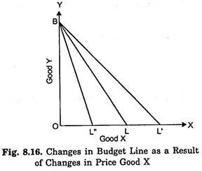
Now, with the lower price of X, the consumer will be able to buy X in greater quantities than before with his given income. Let at the lower price of X, the given income is greater than OL'X to buy OL'. Since the price of Y will remain the same, there will be no change in the purchase volume of good Y with the same given income and there will be no shift to point B as a result. Therefore, if the price of good X falls, the income of consumers 'money and the price of Y remain constant, the price line will take a new position BL'.
Now, what happens to the budget line (initial budget line BL) if the price of good X rises and the price and income of good Y remain unchanged. At a higher price for a good X, consumers can buy a smaller amount of X than before. Therefore, with the increase in the price of X, the price line is assumed to be a new position BL".
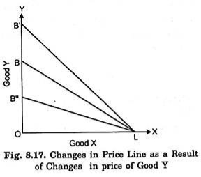
It is a fig. 8.17 indicates the change in the price line when the price of good Y falls or rises, while the price and income of X remain the same. In this case, the initial budget line is BL.A good y price decline, while others remain unchanged, consumers can buy a lot of y with a given money income, thus the budget line will shift to LB', as well as the price y rise, when others are constant, the budget line will shift to LB'.
Changes in income and shifts in budget lines:
Now, the question is what happens to the Y line of the budget if the income changes, while the price of the goods remains the same. The figure shows the effect of changes in income on the budget line. 8.18. Given the specific price of goods and income, let BL be the initial budget line."When a consumer's income increases while the prices of both goods X and Y have not changed, the price line shifts upwards (for example, to B'l') and parallel to the original budget line BL, which means that when income increases, if the whole of income is spent on X, consumers can buy a proportionately greater amount of good X than before, and the whole of income is spent on Y. This is because it is possible to buy a good y in a proportionately larger amount than before. On the other hand, when a consumer's income decreases, the price of both commodity X and commodity X decreases.
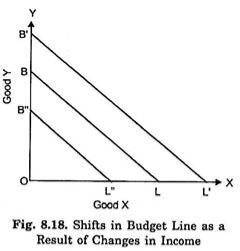
Y remains unchanged, the budget line shifts downward (for example, to B"L"), but remains parallel to the original price line BL. This means that if the whole of the income is spending a change in the income relative to X, if the whole of the income is spending a change in the income relative to X, then the whole of the income is spending a change in the income relative to X.
From above it is clear that the budget line changes when the price of goods changes or the income of consumers changes.
Therefore, the two determinants of the budget line are:
(a) The price of the goods, and
(b) The consumer's income spent on goods;
Two commodity budget lines and price slope:
It is also important to recollect that the slope of the budget line is adequate to the ratio of the worth of two goods. This can be proved with the help of figures. 8.14. Suppose that the given income of the consumer is M, and the given price of the goods X and Y are Px and Py, respectively. The budget line slope BL is OB / OL. I'm going to prove that the slope OB/OL is equal to the ratio of the price of the goods X and Y.
If the whole of the given income M is spent on it, then the amount of good X purchased is OL.

Now, the amount of good Y purchased if the whole of the given income M is spent on it is OB.


Therefore, it has been proven that the slope of the budget line BL represents the ratio of the price of two goods.
Key takeaways - budget lines is important for understanding the idea of consumer equilibrium. The higher apathy curve shows higher satisfaction than the lower one. Therefore, the consumer in his attempt to maximize his satisfaction will try to reach the highest possible indifference curve.
Consumer’s preferences; Interference curve
Consumer preferences
Therefore, the underlying basis of demand may be a model of how consumers behave. This is Individual consumers have a group of preferences and values whose decisions are outside
The area of Economics. They definitely don't depend upon culture, education and individual preferences,
Among a plethora of other factors. The measure of those values during this model is
In terms of real opportunity costs to consumers purchasing and consuming good
If a successful individual purchases a specific product, the chance cost of that purchase are going to be as follows
- Forgone goods that buyers may have bought instead.
- Develop models that map or graphically derive consumer preferences. These are
- Measured in terms of the extent of satisfaction that buyers get from various consumption
- Combination or bundle of products. The aim of the buyer is to pick a bunch of products which offers the very best level of satisfaction as they define it consumer? But consumers they are very constrained in their choice. These constraints are defined by the buyer
- Income and the price that buyers buy goods.
We officially present the model of consumer choice. As we go, we establish a Vocabulary to explain the model. The event of the model is going to be three stages.
After a proper statement of consumer objectives, we map consumer preferences.
Second, we present consumer budget constraints, and eventually, combine the 2 to
Examine the consumer's choice of products.
Consumer theory
Consumers make decisions by allocating their scarce income across all possible commodities.
Get the best satisfaction. Properly speaking, for instance, to maximise the general public interest of Ethiopian consumers to budget constraints utilities are defined because the satisfaction those buyers derive from Consumption of excellent. As mentioned above, the determinant of utility is decided by variety of non-economic factors. The worth of consumers is measured by the relative utility between goods. These reflect consumer preferences.
Theory of consumer preferences
Consumer preferences are defined as subjective (personal) tastes as measured by utilities. Various bundles of products. Goods consistent with their permission a bunch of ranks to consumers. The level of utilities they provide to consumers. Please note that preferences are independent of income Price. The power to shop for goods doesn't determine the likes and dislikes of consumers. One can
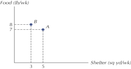
Have a preference for Porsche than Ford, but only have the financial means to drive Ford. These settings are often modelled and mapped using the indifference curve. In order to graphically depict consumer preferences, you would like to define several terms. First, because we will be working in two dimensions (2D graph), we assume two good worlds. These are arbitrary two goods. Common processing defines not only the food, but also the opposite good composite of all other goods. For descriptive simplicity (which makes things easier for me). Define two goods nearly as good X and good Y. The amount of excellent X for horizontal and good Y for vertical. Each point of this Cartesian space then defines some combination of products X and Y.
Product bundle
The goal of the idea of preference is to permit consumers to rank these goods bundle counting on the quantity of usefulness obtained from them. In other words, consumers have different preferences than different combinations of products defined by a group of products.
Assumptions about Preference Orderings
- Integrity: consumers can rank all possible bundles of goods and services.
For any two bundles A and B, the consumer knows whether a is good, B is good, or they are just as good
- Transitivity: for any three bundles a, B, and C, if A is a minimum of nearly as good |pretty much as good"> nearly as good as B and B is a minimum of as good as C, then A is at least as good as C.
- These two assumptions mean the principle of ranking.
The Ranking Principle
Consumers can rank all potentially available choices, in order of preference.
Assumption: More-Is-Better
Others are equal, and better are less preferred.
We ignore harmful or toxic goods that are no better than more but less.
Indifference curve analysis
Utility analysis suffers from a flaw in the subjective nature of utility, that is, the inability to measure utility quantitatively and accurately. To overcome this difficulty, economists developed a different approach based on the indifference curve. According to this indifference curve analysis, utility cannot be accurately measured, but the consumer can state which of the combinations of two goods he prefers, without describing the magnitude of the strength of his preference. This means that if the consumer is presented with a number of different combinations of goods, he can order or rank them on a “scale of preference “if the different combinations are marked a, B, C, D, E, etc. In this case, the consumer can tell whether he likes A to B or B to A or is indifferent between them. Similarly, he can show his preference or indifference between other pairs or combinations. The concept of order utility means that consumers cannot go beyond stating their preferences or indifference. In other words, if consumers prefer A to B, they don't know by “how much “they prefer A to B. Consumers cannot state the “quantitative difference “between different satisfaction levels. He can simply compare them “qualitatively". That is, it is possible to determine whether simply one satisfaction is higher than another, or lower, or equal.
The basic tool of the Hicks-Allen order analysis of demand is the indifference curve, which represents all those combinations of goods that give the consumer the same satisfaction. In other words, all the combinations of goods that lie on the consumer's indifference curve are equally preferred by him. The independence curve is also known as the Iso-utility curve. Indifferent schedules are tabular statements showing different combinations of two goods that bring the same level of satisfaction.
Table 2.4 Indifference schedule
Combination Rice (X) Wheat (Y)

I | 1 | 12 |
II | 2 | 8 |
III | 3 | 5 |
IV | 4 | 3 |
V | 5 | 2 |
Now consumers are asked to tell the amount of wheat (Y) they are willing to give up the benefit of an additional unit of rice (X) so that the level of satisfaction remains the same. If the profit of one unit of rice fully compensates for the loss of 4 units of wheat, then the following combination of 2 units of rice
And eight units of wheat will give him as much
Satisfaction as the first or first combination. A set of indifferent curves representing the size of preference at different levels of satisfaction are understood because the indifferent curve map (figure 2.3).
Although the combination lying on the indifferent curve 3 (IC3) provides the same satisfaction
Product X

Commodity X
Fig 2.3 Indifference Curve Map
Figure 2.3 indifference curve map
The level of satisfaction in the indifference curve 3 (IC3) is greater than the level of
Satisfaction with indifference curve 2(IC2).
I) the nature of the indifference curve
A) Downward inclination: the indifference curve tilts downwards from left to right.
This means that when the amount of one good in a combination increases, the amount of another must necessarily be reduced so that the total satisfaction is constant.
If the indifference curve is a horizontal straight line (parallel to the X-axis),
Then the indifference curve is a horizontal straight line (parallel to the X-axis),
As shown in the figure. 2.4 (a) means that as the amount of good X increases,
The amount of good Y will remain constant, but the consumer will remain
Indifferent among the various combinations.
This cannot be done, because consumers always prefer
a large amount of good to a small amount of its good.
Similarly, the indifference curve cannot be a vertical straight line


 Commodity X Commodity X Commodity X
Fig.2.4 (a) Horizontal Fig.2.4 (b) Vertical Fig.2.4(c) Upward Sloping
Indifference Curve Indifference Curve Indifference Curve
A vertical straight line means that while the amount of good y in combination increases the amount of good X remains constant. The third possibility for the curve is to lean upward to the right.
Consumer’s equilibrium
You are now clear about the indifference curve and budget lines. Next, let's look at the consumer equilibrium. Consumers are in equilibrium when they get maximum satisfaction from the goods and are not in a position to rearrange their purchases. There is a defined apathy map showing the scale of consumer preferences across different combinations of two goods X and Y.
Consumers have a fixed income and want to spend it entirely on goods X and Y.
The price of goods X and Y is fixed to the consumer.
The goods are homogeneous and divisible.
The consumer acts rationally and maximizes his satisfaction.
Consumer equilibrium
Take his indifference curve and budget line together to show the combination of two goods X and Y that consumers buy to be balanced.
We know,
Indifferent map-shows the scale of consumer preferences between various combinations of two goods
Budget line-he shows his money income and various combinations that can afford to buy at the price of both goods.
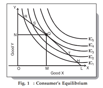
The following figure shows the indifference map with 5 indiscriminate curves (ic1, IC2, IC3, IC4, and IC5) and the budget lines PL for good X and good Y. In order to maximize his level of satisfaction, the consumer tries to reach the highest indifference curve. We assume budget constraints, so he will be forced to stay on the budget line.
So, what kind of combination is it?
Let's say he chose the combination R from the figure. 1, we see that R is on the low indifference curve–IC1. He can easily afford the combination S, Q, or T that is on a high Ic. Even if he chooses the combination H, the argument is similar because H is on the curve IC1.
Next, let's check out the mixture S lying on the curve IC2. Again, he can reach a better level of satisfaction within the budget by choosing the mixture Q lying on IC3–the argument is analogous for the mixture T, since the higher T is also on the curve IC2.
Therefore, we have left the combination Q.
What happens when he chooses the combination Q?
This is the simplest choice because Q is on his budget line and pts puts him on the simplest possible indifference curve, IC3. There are higher curves, IC4 and IC5, but they are over his budget. Thus, he reaches equilibrium at the point Q on the curve IC3.
Note that at this point the budget line PL is bordered by the indifference curve IC3. Also in this position, consumers buy X in OM amount and Y in ON amount.
Since Point Q is tangent, the slope of line PL and curve IC3 is equal at this point. In addition, the slope of the indifference curve shows that the substitution limit rate (MRSxy) of X with respect to Y is
Hence, at the equilibrium point Q,
MRSxy = MUxMUyMUxMUy = PxPy
Also, the slope of the price line (PL) shows the ratio of X and Y prices. Therefore, we can say that the consumer equilibrium is achieved when the price line is bordered by the indifference curve. Alternatively, when the substitution limit rate of goods X and Y is equal to the ratio between the prices of two goods.
Income and substitution effect
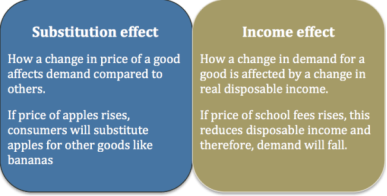
A good increase in prices will then have two different effects–known as profit and alternative effects.
If a good increase in price
- Goods are relatively more expensive than alternatives, and therefore people will switch to other goods that are relatively inexpensive. (Substitution effect)
- Higher prices reduce disposable income, and this low income can reduce demand. (Income effect)
Substitution effect
It states that the increase in the price of good will encourage consumers to buy alternative goods. The alternative effect measures the amount at which higher prices encourage consumers to buy different goods, assuming the same level of income.
Income effect
Thus price changes affect the interests of consumers. If prices rise, it will effectively cut disposable income and lower demand for good for disposable income this fall.
For example:
When the price of meat rises, the higher the price, consumers can switch to alternative food sources, such as buying vegetables.
But the higher the price of meat, it means that after buying some meat, they have a lower reserve income. Therefore, consumers buy less meat, but this profit.
If it goes well, it will increase like a diamond an alternative diamond for no substitution effect however, the higher the price of a diamond, the lower the demand due to the income effect.
Income and alternative effects on wages
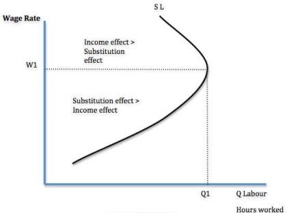
For workers, there is a choice between work and leisure.
When wages rise, work becomes relatively more profitable than leisure time. (Substitution effect)
But with higher wages, he can maintain a decent standard of living through fewer jobs. (Income effect)
The alternative effect of higher pay means workers give up their leisure time to do more hours of work because jobs now have higher rewards.
The income effect of higher wages means that workers spend less time working because they can maintain their target income level in less time.
If the alternative effect is greater than the income effect, people do more work (W1, up to Q1). But we may be at a certain hourly rate where we can afford to work less time. In the figure above, after w1, the income effect is dominant.
It depends on the workers in question. You can enjoy leisure and high-paying jobs. The income effect will soon dominate. If you have a lot of debt and spending commitments, the income effect will take a long time to occur.
Income and alternative effects for interest rates and savings
Higher interest rates increase income from savings. Thus, this will give consumers more income, which can lead to higher spending (income effect)
Higher interest rates make savings more attractive than consumption and reduce consumer spending (alternative effects)
Key takeaways –
- Consumer preferences are defined as subjective (personal) tastes as measured by utilities.
- A good increase in prices will then have two different effects–known as profit and alternative effects.
- Higher interest rates increase income from savings.
REFERENCES
- Karl E. Case and Ray C. Fair, Principles of Economics, Pearson Education Inc., 8th Edition, 2007.
- N. Gregory Mankiw, Economics: Principles and Applications, India edition by South Western, a part of Cengage
- Learning, Cengage Learning India Private Limited, 4th edition, 2007.
- Joseph E. Stiglitz and Carl E. Walsh, Economics, W.W. Norton & Company, Inc., New York, International Student
- Edition, 4th Edition, 2007
- Arthashastra- Dr .Suman