UNIT IV
Closed Economy
4. 0 the Closed Economy in the Short Run
What is a closed economy?
A closed economy has no trading activity with the outside economy. Therefore, a closed economy is completely self-sufficient, meaning that imports do not enter the country and exports do not leave the country. The goal of a closed economy is to provide domestic consumers with everything they need from the border. Why there is no real closed economy
Maintaining a closed economy is difficult in modern society, as raw materials such as crude oil play an important role as inputs to final goods. Many sovereign states do not commonly have raw materials and are forced to import these resources. The closed economy is an instinctive resistance to contemporary liberal economic theory, which promotes the opening of domestic markets to international markets in order to take advantage of comparative advantage and trade.
By focusing on labor and allocating resources to the most productive and efficient work, businesses and individuals can increase their wealth.
Popularization of open trade
Recent globalization means that economies tend to be more open to take advantage of international trade. Petroleum is a good example of a raw material traded worldwide. For example, in 2017, according to World, "sTopExport.com, an independent research and education company, the five largest oil exporters accounted for more than USD $ 841.1 billion in exports.
Saudi Arabia for $ 13.36 billion
$ 93.3 billion Russia
$ 61.5 billion in Iraq
$ 5.4 billion in Canada
United Arab Emirates is $ 49.3 billion.
According to the Energy Information Administration, even the United States, the world's largest oil producer, imported about 104,000 barrels / day in 2017, most of it from Canada, Saudi Arabia, Mexico, Venezuela and Iraq.
Why close the economy?
A fully open economy runs the risk of being overly dependent on imports. Domestic producers can also suffer because they cannot compete at low international prices. Therefore, governments can use trade controls such as tariffs, subsidies and quotas to assist domestic companies.
Closed economies are rare, but governments may shut down certain industries from international competition. Some oil-producing countries have a history of banning foreign oil companies from doing business at their borders.
Example of closed economy
In reality, there is no completely closed economy. Brazil is the world's most closed economy, importing the world's lowest quantity of goods when measured as part of its gross domestic product (GDP). Brazilian companies face competitive challenges such as rising exchange rates and defensive trade policies. In Brazil, only the largest and most efficient companies with large economies can overcome export barriers.
How real interest rates balance commodity markets
Y = C + I (r) + G
Model Background
This model is closed in the sense that the model has no exports or imports. This model includes government taxes and government spending.
If the model is out of equilibrium, it is the changing real interest rate that brings the model back into equilibrium. Y> C + I (r) + G => Interest rate decreases => I is y = C + I (r) + Y <C + I (r) + G => Interest rate increases => I is Y It decreases to = C + I (r) + G.
The left side of the commodity market represents supply
The right side represents demand.

 Supply Y = C + I(r) + G Demand
The classic model was the first attempt to explain:
- Price level determinant
- National level of real GDP
- Employment
- Consumption
- Savings
- Investment
Classical economists-Adam-Smith, J.B. Say, David-Ricardo, John-Stuart-Mill, Thomas-Malthus, A.C. Pigou, etc. wrote in the 1770s and 1930s.
Wages and prices are flexible, assuming there is a competitive market throughout the economy
Say's law
- Economist J.B. Dictates that supply creates its own demand
- Producing goods and services creates the means and motivation to purchase other goods and services.
- Supply makes its demands; therefore it accompanies that the desired spending is equal to the actual spending
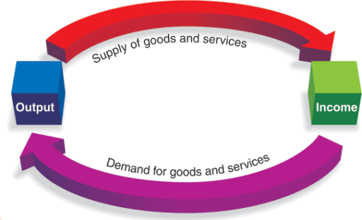
Say’s Law and the Circular Flow
Classic model assumptions
- There is pure competition
- Wages and prices are flexible
- People are motivated by self-interest
- Like gold illusion Gold illusion
- Respond to changes in monetary prices, not relative prices
- If a labour whose wages double when the price level also doubles thinks he or she is better, the labour bears from the false idea of money.
Assumed result
- When the role of government in the economy is minimal;
- When pure competition predominates and all prices and wages are flexible;
- If people are self-interested and have not experienced the illusion of money;
- Then the macroeconomic problem becomes temporary and the market fixes itself
Equilibrium in the credit market
– If income is saved, it will not be reflected in product demand
-Savings are a type of leak from the income and output cycle, as they withdraw funds from the income stream.
-Therefore, the total planned consumption expenditure may be less than the current total real GDP.
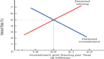
Equating Desired saving and Investment in the Classical Model
Equilibrium in the credit market
- Classic economists argued that each saved dollar was matched by a business investment
- Leakage would thus be equal to injection
- Equilibrium guarantees that the price of credit-interest rate-the amount of credit required is equal to the amount supplied
Equalize the desired preservation and investment of the classic model
- Changes in savings and investment create surpluses or shortfalls in the short term
- In the long run this will be offset by changes in interest rates
- This interest rate adjustment returns the market to the equilibrium of s = I
Question
Will unemployment be a problem with the classic model?
Answer
No, classical economists have assumed that wages will always be adjusted to full employment levels
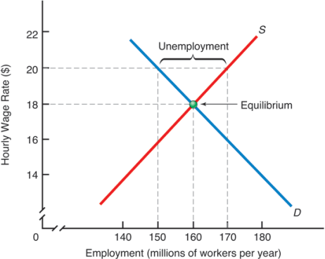
Equilibrium in the Labor Market
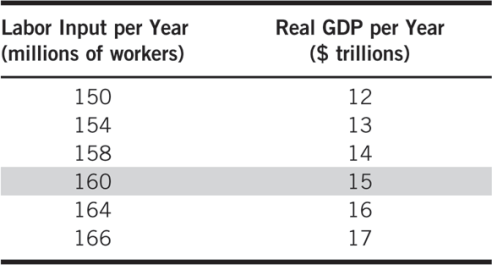
The Relationship between Employment and Real GDP
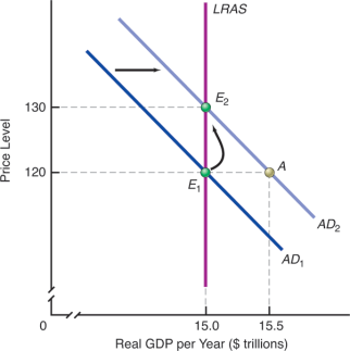
Classical Theory and Increases in Aggregate Demand
Classic theory, vertical total supply and price level
- Long-term unemployment is not possible with the classic model
- Say's Law, along with flexible interest rates, prices and wages, will tend to retain fully employed workers
- LRAS curve is vertical
- Changes in aggregate demand cause changes in price levels

Effect of a Decrease in Aggregate Demand in the Classical Model
The world of classical economists was one of the fully utilized resources
- In the 1930s, Europe and the United States entered an era of economic decline that could not be explained by the classical model.
• John-Maynard-Keynes developed a description that became known as the Keynesian model
• Keynes and his followers insisted
- Prices, including wages (labor prices), are inflexible or "sticky" and downwards
- Aggregate demand, increased advertising will not raise price levels
- Advertising decline does not lower companies price levels
Keynesian short-term aggregate supply curve
Horizontal part of the aggregate supply curve with excessive unemployment and unused capacity in the economy GDP at Less Than Full Employment
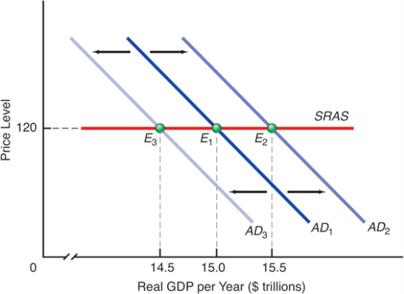
Real GDP and price levels, 1934–1940
- Keynes or the increase in total spending on economic growth without increasing output
- Data showing US recovery from the Great Depression seems to bear this
- In these situations, real GDP is driving demand as the short-term aggregate supply curve was almost flat.
Keynesian model
- Balanced GDP is demand determined
- Keynes Short Aggregate Supply Schedule Shows Source of Price Rigidity
Output Determination Using Aggregate Demand and Aggregate Supply: Fixed versus Changing Price Levels in the Short Run
Trade unions and long-term contracts explain the inflexibility of nominal wage rates
Example: Inflation adjustment
Are US wages "too high"?
The unemployment rate occurs when the labor market is in the black.
If everything else is equal, labor surplus will begin to disappear only if inflation-adjusted wage rates fall towards market clearing levels.
- Since 2008, US inflation-adjusted wages have fallen by about 0.2 percent annually.
- Many economists have suggested that real wages have not fallen enough to eliminate the labor market surplus.
- As a result, a significant number of workers remain unemployed.
• The underlying assumption of the simplified Keynesian model is that the relevant scope of the Short Term Aggregate Supply Schedule (SRAS) is horizontal * Price levels have been in recent decades
Price is not completely sticky
• Modern Keynesian analysis has several
- But not perfect-short-term price adjustments • Short-term aggregate supply curve
- The relationship between total planned economy production and price levels in the short term, everything else was kept constant
- If the price is incompletely adjusted in the short term, the curve is positively sloping
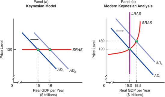
Real GDP Determination with Fixed versus Flexible Prices
In the short term of modern Keynes, a partial rise in price levels can allow real GDP to grow beyond levels consistent with its long-term growth path this is:
-Most employment contracts allow flexibility in the total number of hours worked.
-You can use your existing capital stock harder.
-If wages remain constant when prices rise, firms are more profitable in their business. • All of these adjustments are real GDP as price levels rise:
– Companies use workers more intensively (workers work harder)
-Existing capital equipment used more intensively, (use longer machines)
– If wage rates remain constant, rising price levels will lead to higher profits and lower unemployment as companies hire more.
Shift of aggregate supply curve
The key to non-price levels that can cause shifts in the aggregate supply curve, just as factors in non-price levels can cause shifts in the aggregate demand curve.
Short-term and long-term shifts in total supply
-Includes changes in our donations of production factors
* SRAS shift only
-Including fluctuations in production input prices, especially fluctuations due to temporary external events
Shifts in Long-Run and Short- Run Aggregate Supply
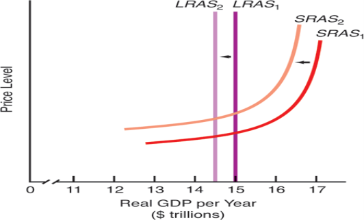
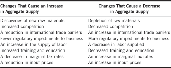
Determinants of Aggregate Supply
International example: Australia's short-term aggregate supply hit by Inagopest
Recently, Australia has experienced the worst locust plague in half a century.
Insects have devastated most of the country's crops, including rice, wheat, barley, and other crops that are livestock feed.
These products are important inputs for many groceries.
The result is a high input price, causing a left shift in aggregate supply.
Consequences of Changes in Aggregate Demand
Aggregate demand shock
-Any event that causes the mixture demand curve to shift inward or outward
Total supply shock
-Events that shift the aggregate supply curve inward or outward
Recession gap
-Gap that exists when the annual equilibrium real GDP is less than the full employment real GDP, as indicated by the position of the Lras curve
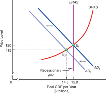
The Short-Run Effects of Stable Aggregate Supply and a Decrease in Aggregate Demand: The Recessionary Gap
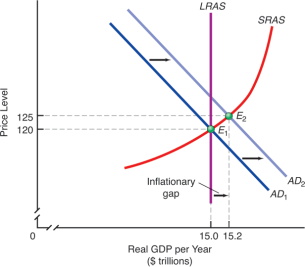
The Effects of Stable Aggregate Supply with an Increase in Aggregate Demand: The Inflationary Gap
Explaining Short-Run Variations in Inflation
* In a growing economy, the explanation for sustainable inflation is that aggregate demand rises over time at a faster pace than full employment levels in real GDP.
* However, short-term fluctuations in inflation can occur as a result of both supply and demand factors.
Demand-Pull-Inflation
– Inflation due to an increase in aggregate demand not matching an increase in aggregate supply
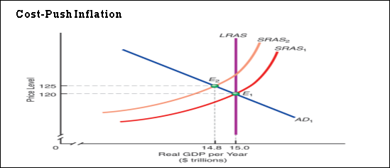
Cost push inflation
-Inflation due to a decrease in short-term aggregate supply
Total supply and demand in the open economy
-Open economy is one of the reasons aggregate demand is declining downwards
-U.S. Residents want to buy cheaper foreign products as domestic price levels rise
– Opposition occurs when price levels in the US fall
When the dollar weakens against other world currencies
-Inward shift to the left on the short-term aggregate supply curve
-Balanced real GDP will fall
-Price levels rise
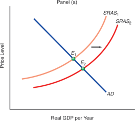 -Employment tends to decrease
-Contribute to inflation
Dollar depreciation, panel ()
• Decreasing the value of dollars incurs the
Cost of imported inputs
- SRAS decreases
- AD constant raises price levels and lowers GDP
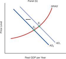
Two effects of the weak dollar, panel (b)
• A decrease within the value of the dollar will increase net exports
* More ads
* With the Sras constant, the price level goes up with GDP
Will the government of the country try to turn off the recession by depressing the exchange value of the country's currency?
• On the one hand, reducing the exchange value of currencies will thereby increase foreign spending on domestic exports and make national export goods cheaper in foreign currencies.
• Meanwhile, the home currency price of inputs imported from abroad will increase.
* Overall, depressing the exchange rate of your home currency does not always help avoid a recession.
You are there: worried about the shock of consolidating supply and demand
• Vincent-Heartnet-Junior, Penski-Logistics president is confused. He hears from the Federal Reserve Board about the fear of deflation. But in his view, inflationary pressure is plentiful:
– His company's medical spending jumped 9% last year
-Fuel costs and wage levels are on the rise
* Therefore, Penske Logistics will associate lower level output with all price levels given.
* He sees this as an indication of rising inflation and has expressed concern that the Federal Reserve could exacerbate the problem.
Challenges and Applications: Measuring the Financial Source of Aggregate Demand Shock
* During the two-week period of 2011, the average value of corporate stocks traded on the US stock market fell by more than 15 percent. This erased about $ 2 trillion in household wealth.
* Households responded by reducing planned spending, resulting in a negative aggregate demand shock.
* The next slide shows the VIX index, which is a measure of financial market volatility.
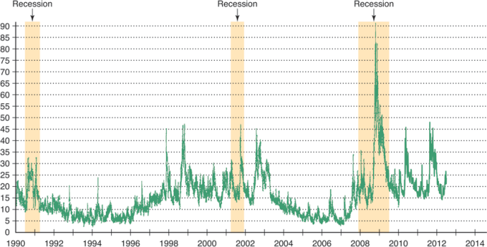
The VIX Index of Financial-Market Volatility since 1990
Challenges and Applications: Measuring the Financial Source of Aggregate Demand Shock
Significant changes in the Vix index can occur due to normal world events or as a result of financial market shocks.
-In 2011, concerns about Greece's financial stability wiped out $ 2 trillion in stock market wealth.
• The recent recession is clearly associated with an increase in the VIX index.
-The financial shock was so great that aggregate demand fell sharply and over the long term.
Central assumptions of the classical model:
1. Pure competition wins
2. Wages and prices are flexible
3. People are motivated by self-interest
4. No money illusion
Short-term establishment of equilibrium real GDP and price levels within the classical model
-In full employment real GDP, the short-term aggregate supply curve is vertical
-In the short term, real GDP cannot increase without changes in the factors of production that drive long-term economic growth.
– Equilibrium price level movements are generated by fluctuations in the position of the ad curve
Situations where the SRA may be tilted horizontally or upwards
-If product prices and wages and other input prices are "sticky", the SRAS curve can be horizontal over most of its range.
-This is the Keynesian SRAS curve
Factors that trigger SRAS and SRAS shifts
LRAS curve
-LRAS shift in response to changes in labor and capital availability, or changes in technology and productivity
– Changes in these factors also cause SRAS
Curve to shift
Impact of aggregate supply and demand shocks on equilibrium real GDP in the short term
A shock that AD shifts to the left and pushes up equilibrium real GDP below full employment real GDP in the short term, so there is a recession gap
Impact of aggregate supply and demand shocks on equilibrium real GDP in the short term
-A shock that causes a rightward shift in the AD curve and causes an inflation gap in which short-term equilibrium real GDP exceeds full employment
Causes of short-term fluctuations in inflation
Demand pull
Increase in aggregate demand
Cost push
Decrease in short-term aggregate supply
Introduction to the Principle of Effective Demand
Before Keynes, no satisfactory explanation was given of the factors determining the level of employment in the economy. Economists mostly assumed the prevalence of the state of full employment by believing in Say's law of markets, an old proposition that states that all income is spent automatically or that the level of effective demand is always sufficient to lift all goods and services. Products from the market.
There were many economists who challenged the assumptions and logic of Say's Law. For example, T.R. Malthus endeavored to convince contemporaries that demand in general may not match supply in general and the shortage of aggregate demand could cause general overproduction and thus general unemployment. But Malthus failed to explain how actual demand could be lacking or excessive. It was Keynes who for the first time proposed a systematic and convincing theory of employment based on the "Principle of Effective Demand". The idea behind this theory is not difficult to grasp.
Keynes’s Principle of Effective Demand:
The principle of "effective demand" underlies Keynes's analysis of income, production and employment. Economic theory was radically changed with the introduction of this principle. In short, the effective demand principle tells us that in the short run, an economy's aggregate income and employment are determined by the level of aggregate demand that is satisfied by aggregate supply. Total employment depends on total demand. As employment increases, income increases. A fundamental principle of the propensity to consume is that as the real income of the community increases, consumption will also increase but less than income.
Therefore, to have enough demand to support an increase in employment, there must be an increase in real investment equal to the gap between income and consumption of that income. In other words, employment can only increase if investment increases. We can generalize and say; a certain level of income and employment can only be maintained if the investment is sufficient to absorb the savings of that level of income. This is the heart of the principle of effective demand.
Meaning of Effective Demand
Effective demand is manifested by the expenditure of income. It is judged by the total expenditure of the economy. The total demand of the economy consists of consumer goods and capital goods, although the demand for consumer goods constitutes a large part of the total demand. Consumption continues to increase with increasing income and employment. At different income levels, there are corresponding demand levels, but not all demand levels are effective. Only that level of demand is efficient which is fully satisfied with the coming supply, so that entrepreneurs do not tend to reduce or increase production.
Effective demand is the demand for production as a whole; in other words, among the different levels of demand, the one that is balanced with the supply in the economy is called effective demand. It is this theory of effective demand that has remained neglected for more than 100 years and has gained importance with the emergence of Keynes's general theory. Keynes was interested in the problem of how much people intended to spend at different levels of income and employment, as it was these planned spending that determined the level of consumption and investment. Keynes' view was that people's spending intentions translated into aggregate demand. If aggregate demand, Keynes said, falls below the income businessmen expect to receive, there will be cuts in the production of goods leading to unemployment. On the contrary, if aggregate demand exceeds expectations, production will be stimulated.
In any community, effective demand represents the money people actually spend on goods and services. The money that entrepreneurs receive flows into the factors of production in the form of wages, rents, interest and profits. In this respect, effective demand (actual expenditure) corresponds to national income, which is the sum of the income of all members of the community. It also represents the value of community production, since the total value of national production is exactly equal to the income of entrepreneurs from the sale of goods. Moreover, all production is either consumer goods or capital goods; we can therefore say that effective demand is equal to national consumer spending plus capital goods.
Effective demand (ED) = national income (Y) = value of national production = expenditure on consumer goods (C) + expenditure on capital goods (I). Hence ED = Y = C + I = 0 = employment.
Importance of the Concept of Effective Demand:
The principle of effective demand is an integral part of Keynesian employment theory. The general theory has the basic observation that aggregate demand determines total employment. A lack of effective demand leads to unemployment. The principle of effective demand is important in the following points. First, it can be said that with the help of the concept of effective demand, Say's market law was rejected. The concept of effective demand has shown beyond any doubt that whatever is produced is not automatically consumed and income is not spent in such a way that the factors of production are fully used. Second, an analysis of effective demand also reveals the inherent contradictions in Pigou's plea that wage cuts will eliminate unemployment. Keynes believes that wage cuts may or may not increase employment as the level of employment depends on the level of real demand.
Third, the effective demand principle could explain how and why depression might persist. Keynes explained that effective demand is consumption and investment. As employment increases, so does income, leading to an increase in consumption, but by less than the increase in income. Thus, consumption lags and becomes the main reason for the gap that exists between total income and total expenditure in order to maintain effective demand at an earlier (or original) level, namely a real investment that corresponds to the gap between income and consumption, it has to be done. In other words, employment can only grow if investment increases. Here the principle of effective demand has the greatest importance. It makes it clear that investments rule the quarter. Fourth, the demand side is moving into the spotlight. In contrast to the classic emphasis on the supply side, Keynes placed great emphasis on the demand side and attributed fluctuations in employment to changes in demand. Effective demand theory illustrates how and why aggregate demand becomes deficient in a capitalist economy, and how a lack of effective demand leads to depression.
Determinants of Effective Demand:
To understand Keynes' employment theory and how employment equilibrium arises in the economy, we need to understand the determinants of the aggregate demand function and the aggregate supply function and their interrelationships.
Aggregate Demand Function and
Aggregate Supply Function.
1. Aggregate Demand Function: The aggregated demand function relates each employment level to the expected revenue from the sale of production from this employment volume. How high the expected sales revenue will be depends on people's expected spending on consumption and investment. Every producer in a free enterprise economy tries to estimate the demand for his product and calculate in advance the profit that will likely be made from his sales proceeds. The total sum of the income payments to the production factors in the production process forms its factor costs. The factor cost and the entrepreneur's profit thus give us the total income or the proceeds that result from a certain amount of employment in a company. Keynes brought this idea into macroeconomics. We can calculate total income or total sales revenue. This total income, or the total revenue expected from a given amount of employment, is called the "total demand price" of the production of that amount of employment; H. It represents expected revenue when employees are offered a certain volume of employment.
Entrepreneurs make decisions about the amount of employment they offer the job based on sales expectations and expected profit, which in turn depend on an estimate of the total money (income) they will get from selling goods that are manufactured at different levels of employment. The sales revenue they expect is the same as what they expect from the community for their production.
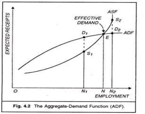
A schedule for the income from the sale of outputs resulting from different levels of employment is called an aggregate demand plan, or aggregate demand node. The total demand function shows the increase in the total demand price with increasing employment and thus increasing production. Thus, the aggregate demand plan is an increasing function of the amount of employment. The question can reasonably be asked: Why did Keynes relate expected sales revenue to employment through manufacturing and why not directly to manufacturing?
Three possible reasons may be given for this:
(i) Keynes was mainly interested in the factors that determine employment rather than production. (ii) Employment and production are moving in all respects in the same direction in a short space of time; (iii) Total production in the economy is made up of a multitude of goods and there is no better measure of it than the labor force employed. If D represents the revenue that entrepreneurs expect from employing N men, the aggregate demand function can be written as D = f (N), which shows a relationship between D and N. The total demand function or the demand plan ADF is shown. We find in the figure that the A dadoes do not start from the origin O, since even with a low level of employment; consumption will be well above income. If we move to the right along the ADF curve, we find that it becomes flatter due to the law of psychological consumption. But the ADF can never fall just because absolute consumption in the economy can never fall.
2. Aggregate Supply Function:
The total offer relates to the production of companies. Entrepreneurs, in providing jobs for workers, need to be sure that the output they produce is sold out and that they are able to meet their production costs and also achieve the expected profit margin. A company's production can be sold at different prices depending on market conditions. However, there is some income from the output for which the entrepreneurs feel that it is only worthwhile to provide a certain amount of jobs. The expected minimum sales revenue of production, which results from a certain amount of employment, is referred to as the "total supply price" of this production. In other words, these are the minimum expected earnings that are seen as only necessary to induce entrepreneurs to provide a certain amount of jobs. For the whole economy at a certain level of employment, the total offer price is the total amount (sales revenue) that all producers together have to expect from the sale of the production produced by that particular number of men, if it is only to be worthwhile to employ.
A schedule of the minimum earnings required to induce entrepreneurs to give different amounts of employment is called a comprehensive pension plan. This is also an increasing function of the amount employed. In other words, the minimum sales revenue requirement continues to rise as employment and output rise. This is due to the increase in production costs with increasing production, since capital, production techniques and organization are taken into account in the short term. It should be noted here that the total demand function is the expected sales revenue that we take into account, and the total supply function is the required minimum sales revenue. There will be a difference between them as at certain levels of employment (outputs) the producers expect more income than the minimum sales revenue required. There will be other levels of employment where the expected sales proceeds may be less than the required sales proceeds.
The aggregate supply function ASF is shown in Figure 4.2 in such a way that it increases gradually and then quickly from left to right. The ASF becomes vertical after point S2, because at this level of the total supply all those who want to be employed receive employment. This point indicates full employment in the economy. Determination of the employment level: In Fig. 4.2 ADF is the aggregate demand function and ASF is the aggregate supply function. We show employment along the X axis and sales revenue along the Y axis. The point E, at which the ADF curve intersects the aggregate supply curve, is called the effective demand point. It can be noted that there are so many points on the aggregate demand curve ADF, but all of these points except for point E are ineffective. In the diagram, the aggregate supply function shows the minimum revenues that are only required to induce entrepreneurs to provide different amounts of employment. The aggregated demand function shows the revenue from the sale of outputs from different employment levels.
Before these curves intersect at E, ASF is below ADF, so that at one level of employment the expected sales revenue N1D1 is higher than the required minimum sales revenue N1S1, which shows that employers are being induced to provide more employment. At point E, ADF is cut through by ASF and the expectations of the entrepreneurs for the proceeds are met. Point E is called the equilibrium point because it determines the actual level of employment (ON) at a given point in time in an economy. The employment level ON2 is not an equilibrium level as the expected sales revenue N2D2 is less than the sales revenue required for N2S2 at this employment level. Most entrepreneurs will be disappointed and reduce employment.
This is how we see it: the intersection of the aggregate demand plan with aggregate supply determines the actual level of employment in an economy, and at that level of employment, the amount of sales revenue that entrepreneurs expect is what they need to get when the cost is at that level of employment just cover. Underemployment Equilibrium: It can be noted, however, that the economy is undoubtedly in equilibrium at time E, since this is where entrepreneurs do not tend to increase or decrease employment. But Keynes makes a unique contribution to economic analysis by saying that E may or may not be a point of full employment equilibrium. If it's so very good.
However, when some workers still remain unemployed after balancing the ADF and ASF, this is known as the underemployment balance. Keynes argued that way. Total demand and total supply could be the same with full employment. This is the case when the investment equals the gap between the total supply price for full employment and the amount that consumers spend on consumption from full employment income. Keynes believed that private investment in a capitalist economy was never enough to fill such a void. Therefore, there is every likelihood that the aggregate demand function and the aggregate supply function will intersect at a point below the underemployment equilibrium known as underemployment. If the underemployment equilibrium is the usual situation in the capitalist economy, then how can we achieve full employment? 7 Keynes suggested that in a short period of time the government could increase aggregate demand in the economy through public investment that was not for profit.
See figure 4.3. Suppose the government makes an investment of D2S2, which raises the ADF to the level of the ADF and the demand function reduces the supply function at S2. The vertical line from point S2 down on the horizontal axis shows that this public investment policy would achieve full employment ON2 in the economy.
Forms of ASF and ADF: It is very difficult to comment on the forms of aggregate demand and supply. Assuming that the money prices of all commodities are constant and that employment and production rise and fall proportionally, we can safely conclude that both the aggregate demand function and the aggregate supply function increase the employment functions; then climb from left to top to the right. The ADF rises quite steeply at first and then flattens out and flattens out. This is because (type of consumption function) MFC is less than one. The ISF rises slowly at first due to the available resources for the unemployed. In view of bottlenecks in production, falling returns (rising costs) are becoming increasingly evident. Beyond full employment, production cannot be increased at all. The sharply rising ASF becomes vertical beyond the full employment point (S2).
Relative Importance of ASF and ADF Functions: Since the equilibrium level of employment is determined by the overlap between these two schedules, it would be useful to learn more details about the nature and nature of these schedules. Of the two, little is important for the aggregate supply function. Keynes pays little attention to the function of total supply and focuses more on the function of total demand. For all practical purposes he takes ASF as given, because he deals with the short time and the delivery conditions cannot be changed in the short time. In addition, Keynes' General Theory dealt with an economy faced with unemployment of resources during the Depression. Under such circumstances, the manipulation of technical production conditions like costs, machines and materials through schemes like rationalization can do little. Rationalization leads to more unemployment in a short time. For these reasons Keynes took ASF for granted.
Since the delivery conditions had to be taken as given. Keynes placed more emphasis on the aggregate demand function. Given the timing of aggregate supply, an economy's resources would only be fully utilized if there is sufficient aggregate demand. It is for this reason that some economists call his theory of employment a "theory of aggregate effective demand". Aggregate demand depends on consumption and investment. If employment is to be developed, consumption and investment spending must be accelerated. Thus, the shape and position of the aggregate demand function depend on the total expenditure incurred by a community for consumption and investment taken together. Assuming, as Keynes describes, the aggregate supply function to be given, the gist of his argument in general theory is that employment is determined by aggregate demand, which in turn depends on the propensity to consume and the amount of the investment at a given time.
Aggregate demand in the statistical sense is composed as follows: (i) Private consumption expenditure, (ii) Private investment expenditure, (iii) Public investment expenditure, iv) External expenditure on national goods and services, in addition to expenditure domestic goods and services. In this way, aggregate demand is a flow of monetary expenditure on final output during a given period. All of these are components of effective demand.
References
- Https://en.m.wikipedia.org/wiki/Macroeconomics
- Principles of Economics by N. Gregory Mankiw
- Foundations of Macroeconomics: Principles, Applications and Tools by Stephen Perez
- A Concise guide to Macro Economics by David A Moss