Module 3
Partial differential equations
A differential equation involving partial derivatives with respect to more than one independent variable is called a partial differential equation.
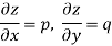
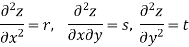
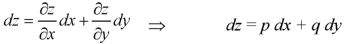
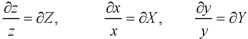
The independent variables will be denoted by x and y and the dependent variable by z. The partial differential coefficients are denoted as-
ORDER of a partial differential equation is the same as that of the order of the highest differential coefficient in it.
Classification of partial differential equation-
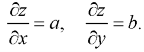
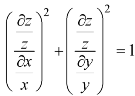
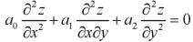
Suppose the equation is-
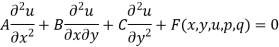
Here A, B, C are the constants of x and y, then the equation-
1. Elliptical- if 
2. Parabolic- if 
3. Hyperbolic- if if 
Formation of partial differential equation-
Method of elimination of arbitrary constants-
Example: Form a partial differential equation from-
Sol.
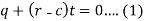
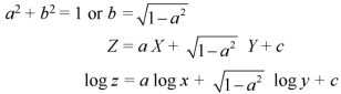
Here we have-
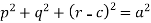
It contains two arbitrary constants a and c
Differentiate the equation with respect to p, we get-
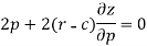
Or
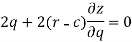
Now differentiate the equation with respect to q, we get-
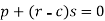
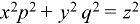
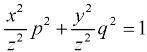
Now eliminate ‘c’,
We get

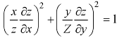
Now put z-c in (1), we get-

Or

The second method we use is method of elimination of arbitrary function.
Solution of partial differential equation by direct partial Integration-
Example: Solve-
Sol.
Here we have-
Integrate w.r.t. x, we get-
Integrate w.r.t. x, we get-
Integrate w.r.t. y, we get-
Example: Solve the differential equation-
Given the boundary condition that-
At x = 0, 
Sol.
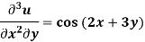
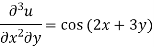
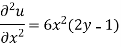
Here we have-
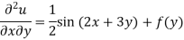
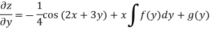
On integrating partially with respect to x, we get-
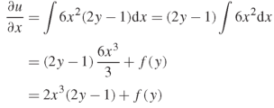
Here f(y) is an arbitrary constant.
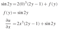
Now form the boundary condition-
When x = 0,

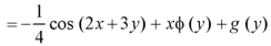
Hence-
On integrating partially w.r.t.x, we get-

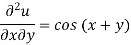
Example: Solve the differential equation-
Given that  when y = 0, and u =
  when x = 0.
Sol.
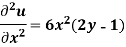
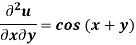
We have-
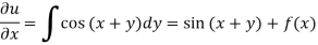
Integrating partially w.r.t. y, we get-
Now from the boundary conditions, 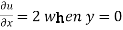
Then-
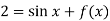
From which,
It means,
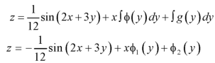
On integrating partially w.r.t. x givens-

From the boundary conditions, u =  when x = 0

From which-
Therefore the solution of the given equation is-

Lagrange’s linear equation in an equation of the type-

Here P, Q and R are the functions of x, y, z and p =  and q =
Working steps to solve-
Step-1: Write down the auxiliary equation-

Step-2: Solve the auxiliary equations-
Suppose the two solutions are- u =  and v =
Step-3: Then f(u, v) = 0 or u = ∅(v) is the required solution of

Method of multipliers-
Let the auxiliary equation be

L, m, n may be the constants of x, y, z then we have-

L, m, n are selected in a such a way that-
Thus
On solving this differential equation, if the solution is- u = 
Similarly, choose another set of multipliers  and if the second solution is v =
So that the required solution is f(u, v) = 0.
Example: Solve-
Sol.
We have-
Then the auxiliary equations are-
Consider first two equations only-


On integrating
 …….. (2)
Now consider last two equations-


On integrating we get-
 …………… (3)
From equation (2) and (3)-
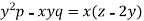
Example: Find the general solution of-
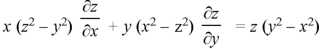
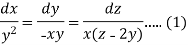
Sol. The auxiliary simultaneous equations are-
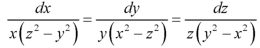 ……….. (1)
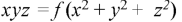
Using multipliers x, y, z we get-
Each term of (1) is equals to-
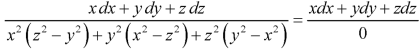
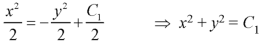
Xdx + ydy + zdz=0
On integrating-
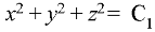 ………… (2)
Again equation (1) can be written as-
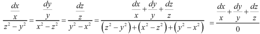
Or
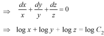
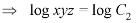
 ………….. (3)
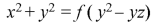
From (2) and (3), the general solution is-
Non-linear partial differential equations-
Type-1: Equation of the type f(p, q) = 0
Method-
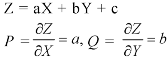
Let the required solution is-
Z = ax + by + c …….. (1)
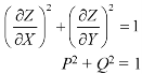
So that-
On putting these values in f(p, q) = 0
We get-
f(a, b) = 0
So from this, find the value of b in terms of a and put the value of b in (1). It will be the required solution.
Type-2: Equation of the type-
Z = px + qy + f(p, q)
Its solution will be-
Z = ax + by + f(a, b)
Type-3: Equation of the type f(z, p, q) = 0
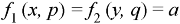
Type-4: Equation of the type-
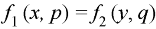
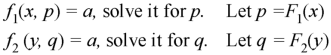
Method-
Let-

Example: Solve-
Sol.
This equation can be transformed as-
 ………. (1)
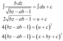
Let

Equation (1) can be written as-
 ………… (2)
Let the required solution be-
From (2) we have-
Example: Solve-
Sol.
Let u = x + by
So that-
Put these values of p and q in the given equation, we get-
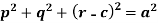
Example: Solve-
Sol.
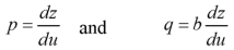
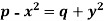
Let-
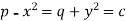
That means-

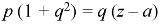
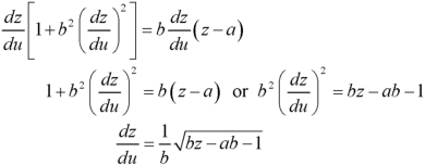
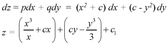
Put these values of p and q in
An equation of the type-
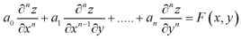
Is called a homogeneous linear partial differential equation of n’th order with constant coefficient.
Rules for finding the complementary functions
Let us consider the equation-
Or
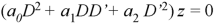
Step-1: Put D = m and D’ = 1
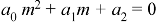
This is the auxiliary equation.
Step-2: Solve the auxiliary equation.
Case-1: If roots of the auxiliary equation are real and different, say 
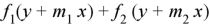
Then C.F.-
Case-2: If roots are equal-
Then C.F.

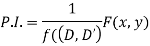
Rules for finding P.I.-
Given partial differential equation is-
f(D, D’)z = F(x, y)
1. When F(x, y) = 
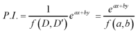
Put D = a and D’ = b
2. When F(x, y) = sin (ax + by) or cos(ax+ by)
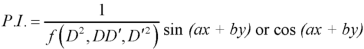
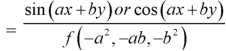
Put 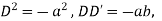
3. When F(x, y) = 
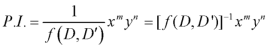
Expand  is ascending power of D and D’ and operate on
  term by term.
4. When F(x,y) any function.
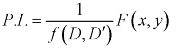
Resolve 1/f(D,D’) into partial fractions.
Considering f(D, D’) as a function of D alone
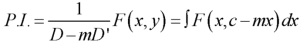
Here c is replaced by y + mx after integration.
Example: Solve-

Sol.
Here we have-

Auxiliary equation will be-

C.F.-
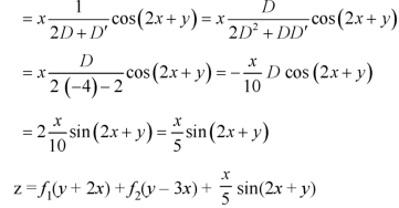
P.I.-
Here

This is the case of failure.
Now-
Example: Solve-
Sol.
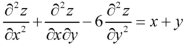
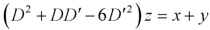
The given equations can be written in the form of-

Its auxiliary equation is-
We get-

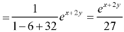
Put D = 1, D’ = 2, -
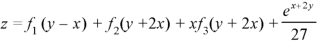
Therefore the complete solution is-
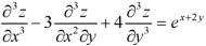
Example: Solve-
Sol.
This equation can be written as-
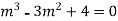
Writing D = m and D’ = 1, then the auxiliary equation will be-
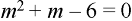
m = -3, 2
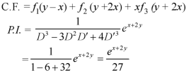
C.F.-
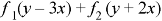
Hence the complete solution is-
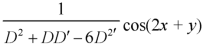
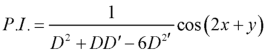
Example: Solve-
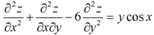
Sol.
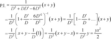
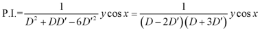
The given partial differential equation can be written in the form-

A.E.-
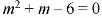
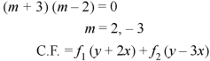
Put y = c + 3x
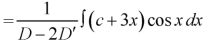

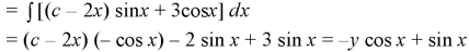
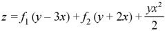
Hence the complete solution is-


