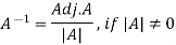
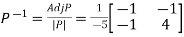
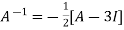
Inverse of a matrix-

The inverse of a matrix ‘A’ can be find as-

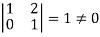
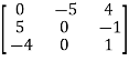
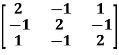
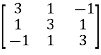
Example: Find the inverse of matrix ‘A’ if-

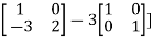
Sol.

Here we have-

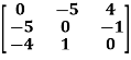
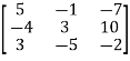
And the matrix formed by its co-factors of |A| is-

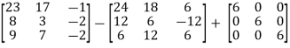
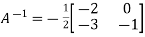
And

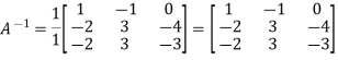
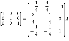
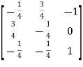
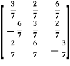
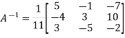
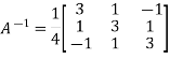
Therefore-

We know that-

Inverse of a matrix by using elementary transformation-

The following transformation are defined as elementary transformations-

1. Interchange of any two rows (column)

2. Multiplication of any row or column by any non-zero scalar quantity k.

3. Addition to one row (column) of another row(column) multiplied by any non-zero scalar.

The symbol ~ is used for equivalence.

Elementary matrices-

If we get a square matrix from an identity or unit matrix by using any single elementary transformation is called elementary matrix.

Note- Every elementary row transformation of a matrix can be affected by pre multiplication with the corresponding elementary matrix.

The method of finding inverse of a non-singular matrix by using elementary transformation-

Working steps-

1. Write A = IA

2. Perform elementary row transformation of A of the left side and I on right side.

3. Apply elementary row transformation until ‘A’ (left side) reduces to I, then I reduces to

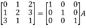
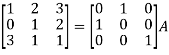
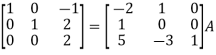
Example-1: Find the inverse of matrix ‘A’ by using elementary transformation-

A =

Sol.  Write the matrix ‘A’ as-  

A = IA

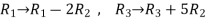
Apply , we get

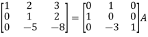
Apply

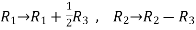
Apply

Apply

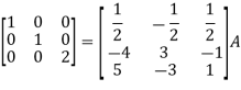
Apply

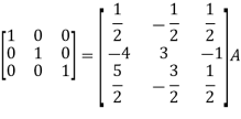
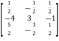
So that,

  =

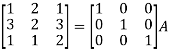
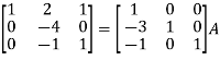
Example-2: Find the inverse of matrix ‘A’ by using elementary transformation-

A =

Sol.  Write the matrix ‘A’ as-  

A = IA

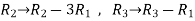
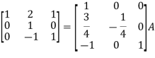
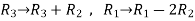
Apply

Apply

Apply

Apply

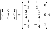
So that

  = 

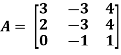
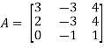
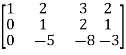
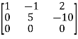
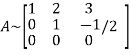
Rank of a matrix-

Rank of a matrix by echelon form-

The rank of a matrix (r) can be defined as –

1. It has at least one non-zero minor of order r.

2. Every minor of A of order higher than r is zero.

Example: Find the rank of a matrix M by echelon form.

M = 

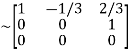
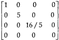
Sol. First we will convert the matrix M into echelon form,

M =

Apply, , we get

M =

Apply  , we get

M =

Apply 

M =

We can see that, in this echelon form of matrix, the number of non – zero rows is 3.

So that the rank of matrix X will be 3.

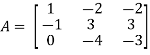
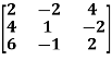
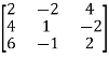
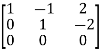
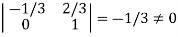
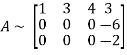
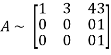
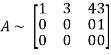
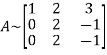
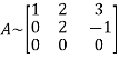
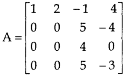
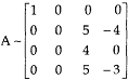
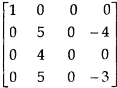
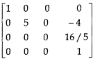
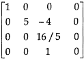
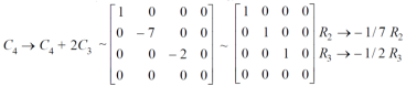
Example: Find the rank of a matrix A by echelon form.

A =

Sol. Convert the matrix A into echelon form,

A =

Apply 

A =

Apply    , we get

A =

Apply , we get

A =

Apply ,

A =

Apply  ,

A =

Therefore, the rank of the matrix will be 2.

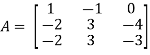
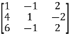
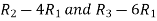
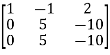
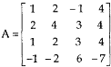
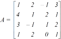
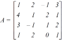
Example:  Find the rank of a matrix A by echelon form.

A =

Sol. Transform the matrix A into echelon form, then find the rank,

We have,

A =

Apply, 

A =

Apply ,

A =

Apply

A =

Apply

A =

Hence the rank of the matrix will be 2.

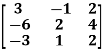
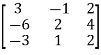
Example:  Find the rank of the following matrices by echelon form?

Let A =

Applying

A 

Applying

A 

Applying

A 

      Applying

A 

It is clear that minor of order 3  vanishes but  minor  of order  2  exists  as 

Hence rank of a given matrix A is 2 denoted by 

2.    

let  A  = 

Applying

Applying

Applying

The minor of   order   3 vanishes but minor of order 2 non zero as 

Hence the rank of matrix A is 2 denoted by

3.    

Let A =

Apply

Apply

Apply

It is clear that the minor of order 3 vanishes where as the minor of order 2 is non zero as 

Hence the rank of given matrix is 2 i.e.

Rank of a matrix by normal form-

Any matrix ‘A’ which is non-zero can be reduced to a normal form of ‘A’ by using elementary transformations.

There are 4 types of normal forms –

The number r obtained is known as rank of matrix A.

Both row and column transformations may be used in order to find the rank of the matrix.

Note-Normal form is also known as canonical form

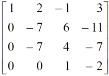
Example: reduce the matrix A to its normal form and find rank as well.

Sol.  We have,

We will apply elementary row operation,

We get,

Now apply column transformation,

We get,

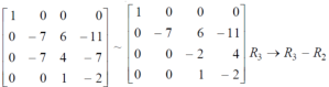
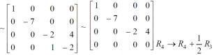
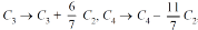
Apply

  , we get,

Apply   and

Apply 

Apply   and

Apply   and

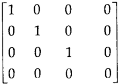
As we can see this is required normal form of matrix A.

Therefore, the rank of matrix A is 3.

Example: Find the rank of a matrix A by reducing into its normal form.

Sol.  We are given,

Apply

Apply

This is the normal form of matrix A.

So that the rank of matrix A = 3

Inverse of a matrix-

1. There are 4 types of normal forms –

2.     Normal form is also known as canonical form

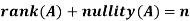
Let A is a matrix of order m by n, then-

Proof: If rank (A) = n, then the only solution to Ax = 0 is the trivial solution x = 0by using invertible matrix.

So that in this case null-space (A) = {0}, so nullity (A) = 0.

Now suppose rank (A) = r < n, in this case there are n – r > 0 free variable in the solution to Ax = 0.

Let represent these free variables and let denote the solution obtained by sequentially setting each free variable to 1 and the remaining free variables to zero.

Here is linearly independent.

Moreover every solution is to Ax  = 0 is a linear combination of

Which shows that spans null-space (A).

Thus is a basis for null-space(A) and nullity (A) = n – r. 

There are two types of linear equations-

1.  Consistent                                   

2. Inconsistent

Let’s understand about these two types of linear equations.

Consistent –

If a system of equations has one or more than one solution, it is said be consistent.

There could be unique solution or infinite solution.

For example-

A system of linear equations-

2x + 4y = 9

x + y = 5

Has unique solution,

Whereas,

A system of linear equations-

2x + y = 6

4x + 2y = 12

Has infinite solutions.

Inconsistent-

If a system of equations has no solution, then it is called inconsistent.

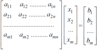
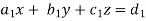
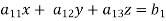
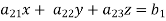
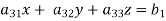
Consistency of a system of linear equations-

Suppose that a system of linear equations is given as-

This is the format as AX = B

Its augmented matrix is-

[A:B] = C

(1) Consistent equations-

If Rank of A = Rank of C

Here, Rank of A = Rank of C = n ( no. of unknown) – unique solution

And Rank of A = Rank of C = r , where r<n   -  infinite solutions

(2) Inconsistent equations-

If Rank of A ≠ Rank of C

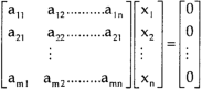
Solution of homogeneous system of linear equations-

A system of linear equations of the form AX = O is said to be homogeneous, where A denotes the coefficients and of matrix and O denotes the null vector.

Suppose the system of homogeneous linear equations is,

It means ,

                             AX = O

Which can be written in the form of matrix as below,

 Note-  A system of homogeneous linear  equations always has a solution if

1. r(A) = n then there will be trivial solution, where n is the number of unknown,

2. r(A) < n , then there will be an infinite number of solution.

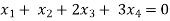
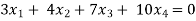
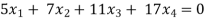
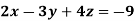
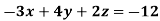
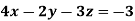
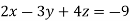
Example: Find the solution of the following homogeneous system of linear equations,

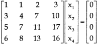
Sol. The given system of linear equations can be written in the form of matrix as follows,

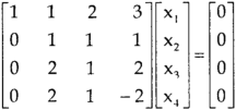
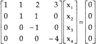
Apply the elementary row transformation,

  , we get,

    , we get

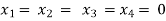
  Here r(A) = 4, so that it has trivial solution,

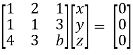
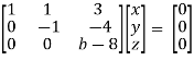
Example: Find out the value of ‘b’ in the system of homogenenous equations-

2x + y + 2z = 0

x + y + 3z = 0

4x + 3y +  bz = 0

Which has

(1) Trivial solution

(2) Non-trivial solution

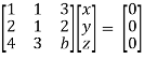
Sol. (1)

For trivial solution, we already know that the values of x , y and z will be zerp, so that ‘b’ can have any value.

Now for non-trivial solution-

(2)

Convert the system of equations into matrix form-

AX = O

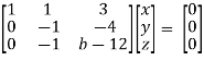
Apply Respectively , we get the following resultant matrices

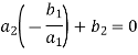
For non-trivial solutions, r(A) = 2 < n

b – 8 = 0

b = 8

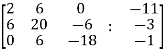
Solution of non-homogeneous system of linear equations-

Example-1: check whether the following system of linear equations is consistent of not.

2x + 6y = -11

6x + 20y – 6z = -3

6y – 18z = -1

Sol. Write the above system of linear equations in augmented matrix form,

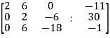
Apply , we get

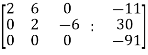
Apply

Here the rank of C is 3 and the rank of A is 2

Therefore, both ranks are not equal. So that the given system of linear equations is not consistent.

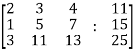
Example: Check the consistency and find the values of x , y and z of the following system of linear equations.

2x + 3y + 4z = 11

X + 5y + 7z = 15

3x + 11y + 13z = 25

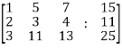
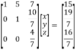
Sol. Re-write the system of equations in augmented matrix form.

                                  C = [A,B] 

That will be,

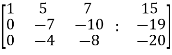
Apply 

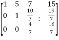
Now apply,

We get,

~~

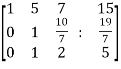
Here rank of A = 3

And rank of C = 3, so that the system of equations is consistent,

So that we can can solve the equations as below,

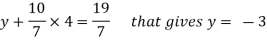
That gives,

x + 5y + 7z = 15  ……………..(1)

y + 10z/7 = 19/7 ………………(2)

4z/7 = 16/7 ………………….(3)

From eq. (3)

z = 4,

From 2,

From eq.(1), we get

x + 5(-3) + 7(4) = 15

That gives,

x = 2

Therefore the values of x , y , z are    2 , -3 , 4  respectively.

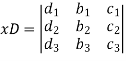
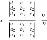
Cramer’s rule-

This method was introduced by Gabriel Cramer (1704 – 1752).

Suppose we have to solve the following equations,

Now, let-

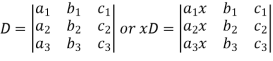
Multiply the second column by y and 3rd column by z and adding to the first column then we have-

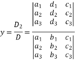
Similarly we get-

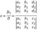
And

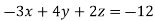
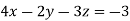
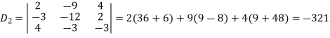
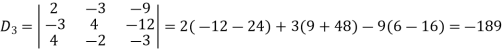
Example: Solve the following equations by using Cramer’s rule-

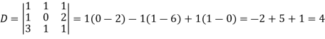
Sol.

Here we have-

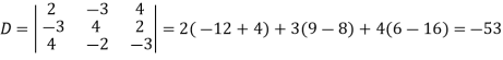
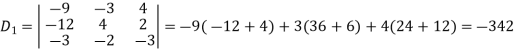
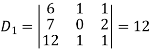
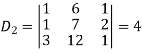
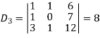
And here-

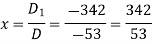
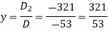
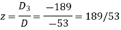
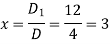
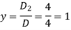
Now by using cramer’s rule-

Example: Solve the following system of linear equations-

Sol.

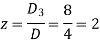
By using cramer’s rule-

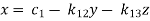
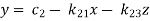
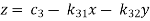
Gauss-Seidel iteration method-

Step by step method to solve the system of linear equation by using Gauss Seidal Iteration method-

Suppose,

This system can be written as after dividing it by suitable constants,

Step-1 Here put y = 0 and z = 0  and x = in first equation

Then in second equation we put this value of x that we get the value of y.

In the third eq. we get z by using the values of x and y

Step-2: we repeat the same procedure

Example: solve the following system of linear equations by using Guassseidel method-

6x + y + z = 105

4x + 8y + 3z = 155

5x + 4y  - 10z = 65

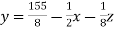
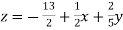
Sol. The above equations can be written as,

   ………………(1)

………………………(2)

   ………………………..(3)

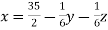
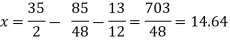
Now put z = y = 0 in first eq.

We get

x = 35/2

put x = 35/2 and z = 0 in eq. (2)

we have,

Put the values of x and y in eq. 3

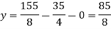
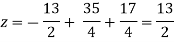
Again start from eq.(1)

By putting the values of y and z

y = 85/8 and z = 13/2

We get

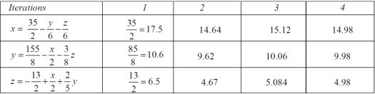
The process can be showed in the table format as below

At the fourth iteration, we get the values of x = 14.98 , y = 9.98  , z = 4.98

Which are approximately equal to the actual values

As x = 15  , y = 10 and  y = 5 ( which are the actual values)

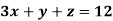
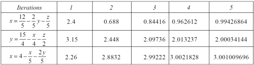
Example: Solve the following system of linear equations by using Guassseidel method-

5x + 2y  + z = 12

x + 4y + 2z = 15

x + 2y + 5z = 20

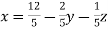
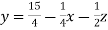
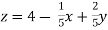
sol. These equations can be written as ,

   ………………(1)

………………………(2)

   ………………………..(3)

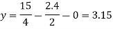
Put y and z equals to 0 in eq. 1

We get,

x = 2.4

put x = 2.4, and z = 0 in eq. 2 , we get

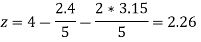
Put x = 2.4 and y = 3.15 in eq.(3) , we get

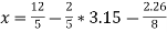
Again start from eq.(1), put the values of y and z , we get

= 0.688

We repeat the process again and again ,

The following table can be obtained –

We see that the values are approx. equal to exact values.

Exact values are, x = 1, y = 2,   z = 3.

Symmetric matrix:

Any square matrix is said to be symmetric matrix if its transpose equals to the matrix itself.

For example:

&

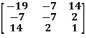
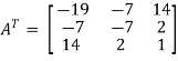
Example: check whether the following matrix A is symmetric or not?

A = 

Sol. As we know that if the transpose of the given matrix is same as the matrix itself then the matrix is called symmetric matrix.

So that, first we will find its transpose,

Transpose of matrix A ,

Here,

A =

So that, the matrix A is symmetric.

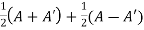
Example: Show that any square matrix can be expressed as the sum of symmetric matrix and anti- symmetric matrix.

Sol.  Suppose A is any square matrix.

Then,

A =

Now,

(A + A’)’ = A’ + A

A+A’ is a symmetric matrix.

Also,

(A - A’)’ = A’ – A

Here A’ – A is an anti – symmetric matrix

So that,

Square matrix = symmetric matrix + anti-symmetric matrix

Skew-symmetric matrix-

A square matrix A is said to be skew symmetrix matrix if –

1. A’ = -A,    [ A’ is the transpose of A]

2. All the main diagonal elements will always be zero.

For example-

A =

This is skew symmetric matrix, because transpose of matrix A is equals to negative A.

Example: check whether the following matrix A is symmetric or not?

A =

Sol. This is not a skew symmetric matrix, because the transpose of matrix A is not equals to -A.

-A = A’

Orthogonal matrix-

Any square matrix A is said to be an orthogonal matrix if the product of the matrix A and its transpose is an identity matrix.

Such that,

A. A’ = I

Matrix × transpose of matrix = identity matrix

Note- if |A| = 1, then we can say that matrix A is proper.

Examples:                 and              are the form of orthogonal matrices.

Look at the following procedure in order to understand the concept of determinants-

Let’s consider the two linear equations,

From first eq. , we get,

Put this value in second equation, we get

This can be written as,

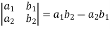
The expansion of the determinant is given as,

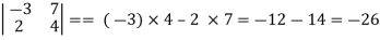
Example: expand the determinant

Sol. As we know, expansion of the determinant is given by,

Then we get,

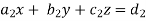
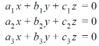
Now suppose we have three equations as below, where a, y and z are unknown,

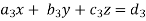
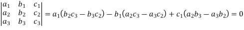
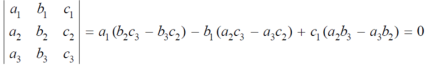
Then the determinant will be of third order and can be defined as follows,

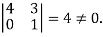
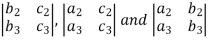
Minor –

The minor of an element is define as determinant obtained by deleting the row and column containing the element.

In a determinant,

The minor of are given by

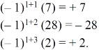
Cofactor –

Cofactors can be defined as follows,

                          Cofactor = minor

Where r is the number of rows and c is the number of columns.

Example: Find the minors and cofactors of the first row of the determinant.

Sol.  (1)  The minor of element 2 will be,

Delete the corresponding row and column of element 2,

We get,

Which is equivalent to,     1 × 7 - 0 × 2 = 7 – 0 = 7

Similarly the minor of element 3 will be,  

4× 7 - 0× 6 = 28 – 0 = 28

Minor of element 5,  

4 × 2 - 1× 6 = 8 – 6 = 2

The cofactors of 2, 3 and 5 will be,

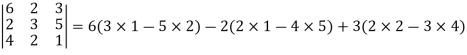
Example: expand the determinant:

Sol. As we know

Then,                         

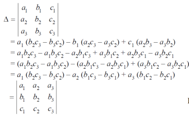
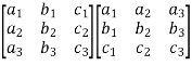
Properties of determinants-

(1) If the rows are interchanged into columns or columns into rows then the value of determinants does not change.

Let us consider the following determinant:

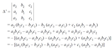
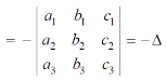
(2) The sign of the value of determinant changes when two rows or two columns are interchanged.

Interchange the first two rows of the following, we get

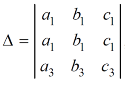
(3) If two rows or two columns are identical the the value of determinant will be zero.

Let, the determinant has first two identical rows,

As we know that if we interchange the first two rows then the sign of the value of the determinant will be changed , so that

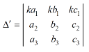
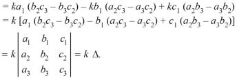
     Hence proved

(4) if the element of any row of a determinant be each multiplied by the same number then the determinant multiplied by the same number,

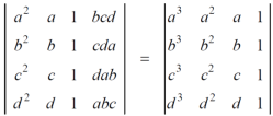
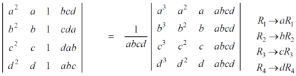
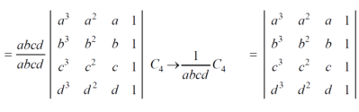
Example: prove the following without expanding the determinant.

 Sol.  Here in order to prove the above result, we follow the steps below,

hence proved.

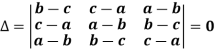
Example: prove that (without expanding) the determinant given below is equal zero.

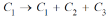
Sol.  Applying the operation,

        We get,

Now applying the operation,

We get,

Apply,

We get,

Here first and second row are identical then we know that by property it becomes zero.             

Example: Show that,

Sol.  Applying

          We get,

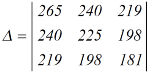
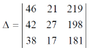
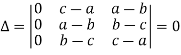
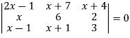
Example: Solve-

Sol:

given-

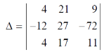
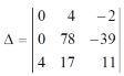
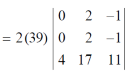
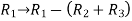
Apply-

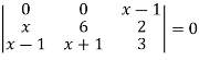
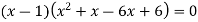
We get-

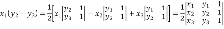
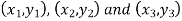
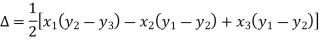
Applications of determinants-

Determinants have various applications such as finding the area and condition of collinearity.

Area of triangles-

Suppose the three vertices of a triangle are respectively, then we know that the area of the triangle is given by-

This is how we can find the area of the triangle.

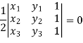
Condition of collinearity-

Let there are three points

Then these three points will be collinear if -

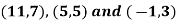
Example: Show that the points given below are collinear-

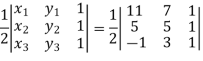
Sol.

First we need to find the area of these points and if the area is zero then we can say that these are collinear points-

So that-

We know that area enclosed by three points-

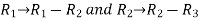
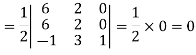
Apply-

So that these points are collinear.

1. 
2. In a determinant,

The minor of are given by

3.     Cofactor –

Cofactors can be defined as follows,

                          Cofactor = minor

Where r is the number of rows and c is the number of columns.

4.     Area of triangles-

5.     Condition of collinearity-

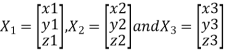
First we will go through some important definitions before studying Eigen values and Eigen vectors.

1. Vector-

An ordered n – touple of numbers is called an n – vector. Thus the ‘n’ numbers x1, x2, …………xn taken in order denote the vector x. i.e. x = (x1, x2, ……., xn).

Where the numbers x1, x2, ………..,xn are called component or co – ordinates of a vector x. A vector may be written as row vector or a column vector.

If A be an mxn matrix then each row will be an n – vector & each column will be an m – vector.

2. Linear dependence-

A set of n – vectors. x1, x2, …….., xr is said to be linearly dependent if there exist scalars. k1, k2, …….,kr not all zero such that

k1 + x2k2 + …………….. + xrkr = 0     … (1)

3. Linear independence-

A set of r vectors x1, x2, ………….,xr is said to be linearly independent if there exist scalars k1, k2, …………, kr all zero such that

x1 k1 + x2 k2 + …….. + xrkr = 0

Important notes-

1. Equation (1) is known as a vector equation.
2. If the vector equation has non – zero solution i.e. k1, k2, ….,kr not all zero. Then the vector x1, x2, ……….xr are said to be linearly dependent.
3. If the vector equation has only trivial solution i.e.

k1 = k2 = …….=kr = 0. Then the vector x1, x2, ……,xr are said to linearly independent.

4. Linear combination-

A vector x can be written in the form.

x = x1 k1 + x2 k2 + ……….+xrkr

where k1, k2, ………….., kr are scalars, then X is called linear combination of x1, x2, ……, xr.

Results:

1. A set of two or more vectors are said to be linearly dependent if at least one vector can be written as a linear combination of the other vectors.
2. A set of two or more vector are said to be linearly independent then no vector can be expressed as linear combination of the other vectors.

Example 1

Are the vectors , , linearly dependent. If so, express x1 as a linear combination of the others.

Solution:

Consider a vector equation,

i.e.

Which can be written in matrix form as,

Here & no. of unknown 3. Hence the system has infinite solutions. Now rewrite the questions as,

Put

and

Thus

i.e.

i.e.

Since F11k2, k3 not all zero. Hence are linearly dependent.

Example 2

Examine whether the following vectors are linearly independent or not.

and .

Solution:

Consider the vector equation,

i.e.   … (1)

Which can be written in matrix form as,

R12

R2 – 3R1, R3 – R1

R3 + R2

Here Rank of coefficient matrix is equal to the no. of unknowns. i.e. r = n = 3.

Hence the system has unique trivial solution.

i.e.

i.e. vector equation (1) has only trivial solution. Hence the given vectors x1, x2, x3 are linearly independent.

Example 3

At what value of P the following vectors are linearly independent.

Solution:

Consider the vector equation.

i.e.

This is a homogeneous system of three equations in 3 unknowns and has a unique trivial solution.

If and only if Determinant of coefficient matrix is non zero.

consider .

.

i.e.

Thus for the system has only trivial solution and Hence the vectors are linearly independent.

Note:

If the rank of the coefficient matrix is r, it contains r linearly independent variables & the remaining vectors (if any) can be expressed as linear combination of these vectors.

Characteristic equation:

Let A he a square matrix, be any scalar then is called characteristic equation of a matrix A.

Note:

Let a be a square matrix and ‘’ be any scalar then,

1)     is called characteristic matrix

2)     is called characteristic polynomial.

The roots of a characteristic equations are known as characteristic root or latent roots, Eigen values or proper values of a matrix A.

Eigen vector:

Suppose be an Eigen value of a matrix A. Then a non – zero vector x1 such that.

     … (1)

Such a vector ‘x1’ is called as Eigen vector corresponding to the Eigen value .

Properties of Eigen values:

1. Then sum of the Eigen values of a matrix A is equal to sum of the diagonal elements of a matrix A.
2. The product of all Eigen values of a matrix A is equal to the value of the determinant.
3. If are n Eigen values of square matrix A then are m Eigen values of a matrix A-1.
4. The Eigen values of a symmetric matrix are all real.
5. If all Eigen values are non –zero then A-1 exist and conversely.
6. The Eigen values of A and A’ are same.

Properties of Eigen vector:

1. Eigen vector corresponding to distinct Eigen values are linearly independent.
2. If two are more Eigen values are identical then the corresponding Eigen vectors may or may not be linearly independent.
3. The Eigen vectors corresponding to distinct Eigen values of a real symmetric matrix are orthogonal.

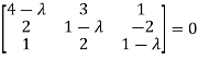
Example-1:

Determine the Eigen values of Eigen vector of the matrix.

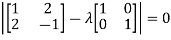
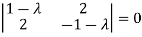
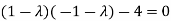
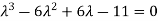
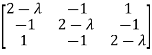
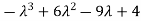
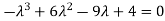
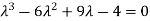
Solution:

Consider the characteristic equation as,

i.e.

i.e.

i.e.

Which is the required characteristic equation.

are the required Eigen values.

Now consider the equation

        … (1)

Case I:

If   Equation (1) becomes

R1 + R2

Thus

independent variable.

Now rewrite equation as,

Put x3 = t

&

Thus .

Is the eigen vector corresponding to .

Case II:

If equation (1) becomes,

Here

Independent variables

Now rewrite the equations as,

Put

&

.

Is the eigen vector corresponding to .

Case III:

If equation (1) becomes,

Here rank of

independent variable.

Now rewrite the equations as,

Put

Thus .

Is the eigen vector for .

Example 2

Find the Eigen values of Eigen vector for the matrix.

Solution:

Consider the characteristic equation as

i.e.

i.e.

are the required eigen values.

Now consider the equation

       … (1)

Case I:

Equation (1) becomes,

Thus and n = 3

3 – 2 = 1 independent variables.

Now rewrite the equations as,

Put

,

I.e.

the Eigen vector for

Case II:

If equation (1) becomes,

Thus

Independent variables.

Now rewrite the equations as,

Put

Is the Eigen vector for

Now

Case III:

If equation (1) gives,

R1 – R2

Thus

Independent variables

Now

Put

Thus

Is the Eigen vector for

Two square matrix and A of same order n are said to be similar if and only if

for some non singular matrix P.

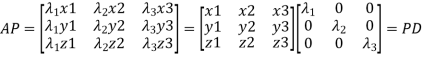
Such transformation of the matrix A into with the help of non singular matrix P is known as similarity transformation.

Similar matrices have the same Eigen values.

If X is an Eigen vector of matrix A then is Eigen vector of the matrix

Reduction to Diagonal Form:

Let A be a square matrix of order n has n linearly independent Eigen vectors Which form the matrix P such that

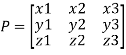
Where P is called the modal matrix and D is known as spectral matrix.

Procedure: let A be a square   matrix of order 3.

Let three Eigen vectors of A are  Corresponding to Eigen values

Let     

  {by characteristics equation of A}

Or

Or 

Note: The method of diagonalization is helpful in calculating power of a matrix.

  .Then for an integer n we have  

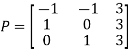
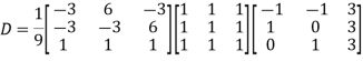
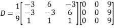
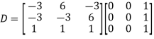
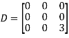
We are using the example of 1.6*

Example1:  Diagonalise the matrix

Let A=

The three Eigen vectors obtained are  (-1,1,0), (-1,0,1) and (3,3,3) corresponding to Eigen values .

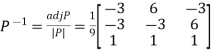
Then    and

Also we know that    

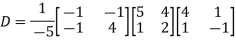
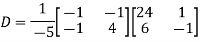
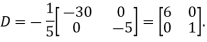
Example2: Diagonalise the matrix

Let A =

The Eigen vectors are (4,1),(1,-1) corresponding to Eigen values .

Then    and also 

Also we know that    

1. Two square matrix and A of same order n are said to be similar if and only if

for some non singular matrix P.

2.     Let A be a square matrix of order n has n linearly independent Eigen vectors Which form the matrix P such that

Where P is called the modal matrix and D is known as spectral matrix.

Statement-

Every square matrix satisfies its characteristic equation , that means for every square matrix of order n,

|A - | =

Then the matrix equation-

Is satisfied by X = A

That means

Example-1: Find the characteristic equation of the matrix A =   and Verify cayley-Hamlton theorem.

Sol. Characteristic equation of the matrix, we can be find as follows-

Which is,

( 2 -  , which gives

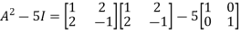
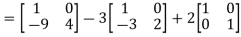
According to cayley-Hamilton theorem,

  …………(1)

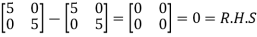
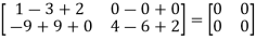
Now we will verify equation (1),

Put the required values in equation (1) , we get

Hence the cayley-Hamilton theorem is verified.

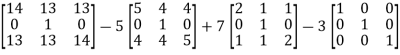
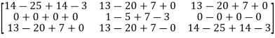
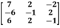
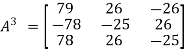
Example-2: Find the characteristic equation of the the matrix A and verify Cayley-Hamilton theorem as well.

A =

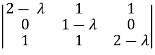
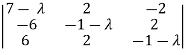
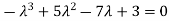
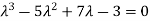
 Sol. Characteristic equation will be-

= 0

( 7 -

(7-

(7-

Which gives,

Or

According to cayley-Hamilton theorem,

   …………………….(1)

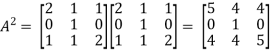
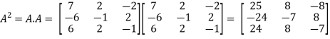
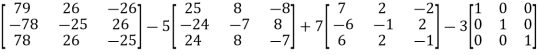
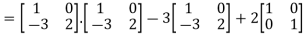
In order to verify cayley-Hamilton theorem , we will find the values of 

So that,

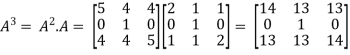
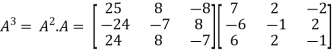
Now

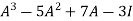
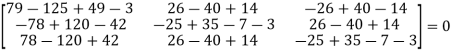
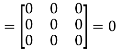
Put these values in equation(1), we get

= 0

Hence the cayley-hamilton theorem is verified.

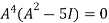
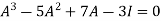
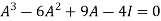
Example-3:Using Cayley-Hamilton theorem, find , if A = ?

Sol. Let A =

The characteristics equation of A is

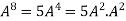
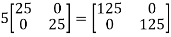
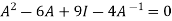
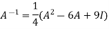
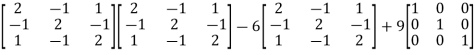
Or

Or

By Cayley-Hamilton theorem   

L.H.S.

=

By Cayley-Hamilton theorem we have   

            Multiply both side by

.

Or 

=

=

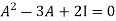
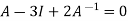
Inverse of a matrix by Cayley-Hamilton theorem-

We can find the inverse of any matrix by multiplying the characteristic equation With .

For example, suppose we have a characteristic equation   then multiply this by  , then it becomes

Then we can find by solving the above equation.

Example-1: Find the inverse of matrix A by using Cayley-Hamilton theorem.

A =

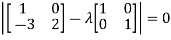
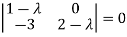
Sol.  The characteristic equation will be,

|A - | = 0

Which gives,

(4-

According to Cayley-Hamilton theorem,

Multiplying by 

That means

On solving,

11

= 

= 

So that,

Example-2: Find the inverse of matrix A by using Cayley-Hamilton theorem.

                                            A =

Sol.  The characteristic equation will be,

|A - | = 0

= 

= (2-

= (2 -

=

That is,

Or

We know that by Cayley-Hamilton theorem,

…………………….(1)t,

Multiply equation(1) by , we get

Or

Now we will find 

=

=

Hence the inverse of matrix A is,

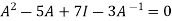
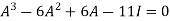
Example-3: Verify the Cayley-Hamilton theorem and find the inverse.

?

Sol.  Let A =

The characteristics equation of A is

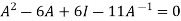
Or

Or 

Or 

By Cayley-Hamilton theorem 

                                   L.H.S:

                                                 =   =0=R.H.S

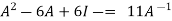
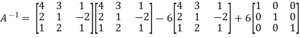
Multiply both side by on 

                                               Or

                                              Or [

                                               Or

Orthogonal transformation-

When a transformation from one set of rectangular coordinates to another set of rectangular coordinates  , then this is called ‘orthogonal tranformation’.

In other words-

A linear transformation Y = AX is said to be orthogonal , if matrix A is orthogonal that means,

                         AA’ = I = A’A

We have,

And similarly,

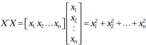
If Y = AX is an orthogonal transformation , then we have

        X’X = Y’Y = (AX)’AX = X’A’ AX = X’(A’A)X

Which is only possible , if

A’A = I = AA’  and

Therefore the square matrix A is said to be orthogonal if AA’ = A’A and

Example: Check whether the matrix A is orthogonal or not?

                              A =

Sol. To check the orthogonality of this matrix , first we need to find AA’

So that,

        AA’ =

               =

Here AA’ ≠ I

So , we can say that matrix A is not an orthogonal matrix.

Example: If the matrix A defines an orthogonal transformation , then show that

+    ( i≠j)  i,j = 1 , 2 , 3.

Where            A =

Sol.  As we know that an orthogonal matrix A ,

               AA’ = I = A’A     and 

We will find AA’,

        AA’ =   =

A will be orthogonal only if -    AA’ = I

In that case, it is only possible when,

= = 1

And,

() = () = () = 0

NOTES-

1. The inverse and transpose of an orthogonal matrix is also orthogonal.

2. A linear transformation preserves length if and only if its matris is orthogonal.

3. The product of two or more than two orthogonal matrices is also orthogonal.

4. The determinant of an orthogonal matrix will always be ±1.

1. 
2. Orthogonal transformation-

When a transformation from one set of rectangular coordinates to another set of rectangular coordinates  , then this is called ‘orthogonal tranformation’.

References

- E. Kreyszig, “Advanced Engineering Mathematics”, John Wiley & Sons, 2006.
- P. G. Hoel, S. C. Port And C. J. Stone, “Introduction To Probability Theory”, Universal Book Stall, 2003.
- S. Ross, “A First Course in Probability”, Pearson Education India, 2002.
- W. Feller, “An Introduction To Probability Theory and Its Applications”, Vol. 1, Wiley, 1968.
- N.P. Bali and M. Goyal, “A Text Book of Engineering Mathematics”, Laxmi Publications, 2010.
- B.S. Grewal, “Higher Engineering Mathematics”, Khanna Publishers, 2000.
- T. Veerarajan, “Engineering Mathematics”, Tata Mcgraw-Hill, New Delhi, 2010
- Higher engineering mathematics, HK Dass